Application of PageRank algorithm to analyze packages in R

Introduction

In the previous article, we talked about a crucial algorithm named PageRank, used by most of the search engines to figure out the popular/helpful pages on web. We learnt that however, counting the number of occurrences of any keyword can help us get the most relevant page for a query, it still remains a weak recommender system.

In this article, we will take up some practice problems which will help you understand this algorithm better. We will build a dependency structure between R packages and then try to solve a few interesting puzzles using PageRank algorithm. But before we do that, we should brush up our knowledge on packages in R for better understanding.

Packages in R

R is language built on top of many different packages. These packages contain user-ready functions which make our job easier to do any kind of statistical analysis. These packages are dependent on each other.

For instance, a statistical package like Random Forest is dependent on many packages to seek help in evaluating multiple statistical parameters. Before going into dependency structures, let’s learn a few commands on R :

miniCran : Many private firms like to create a mirror image of all the packages R has to offer on their own server. This package “miniCran” helps these firms to create a subset of packages required. But why do we even need a package to create a mirror image?

The reason is that there is a complex structure between these packages of dependencies. These dependencies tell R which package should get installed before installing a new package. “miniCran” is like a blueprint of all these packages.

Function “pkgDep” : This is a magic function which will bring out all the dependencies for a package. There are three different types of dependencies between packages. Let’s understand these three:

• Imports : This is the most important dependency. It is a complete package with its recursive dependencies required to be installed first.
• Suggests : This means that the dependency is restricted to a few functions and hence do not need recursive rights.
• Enhances : This means that the current package adds something to another package and no recursive dependency is required.

Let’s now try our hand on a few package dependency structures:

library(miniCRAN)
pkgs <- "ggplot2"
pkgDep(pkgs, suggests=FALSE, enhances=FALSE, includeBasePkgs = TRUE)

[1] "ggplot2" "chron" "stats" "methods" "plyr"  "digest" "grid" "gtable" "reshape2" "scales" 
[11] "proto" "MASS" "grDevices" "graphics" "utils"  "Rcpp" "stringr" "RColorBrewer" "dichromat" "munsell" "labeling" "colorspace"

pkgDep(pkgs, suggests=TRUE, enhances=FALSE, includeBasePkgs = TRUE)

[1] "ggplot2" "chron" "stats" "methods" "plyr"  "digest" "grid" "gtable" "reshape2" "scales" 
[11] "proto" "MASS" "grDevices" "graphics" "utils" "Rcpp" "stringr" "RColorBrewer" "dichromat" "munsell" "labeling" "colorspace" "SparseM" "lattice" "survival" "Formula" "latticeExtra" "cluster" "rpart" "nnet" "acepack" "foreign" "splines" "maps" "sp" "mvtnorm" "TH.data" "sandwich" "codetools" "zoo" "evaluate" "formatR" "highr" "markdown" "tools"  "mime" "nlme" "Matrix" "quantreg" "Hmisc" "mapproj" "hexbin" "maptools" "multcomp" "testthat" "knitr" "mgcv"

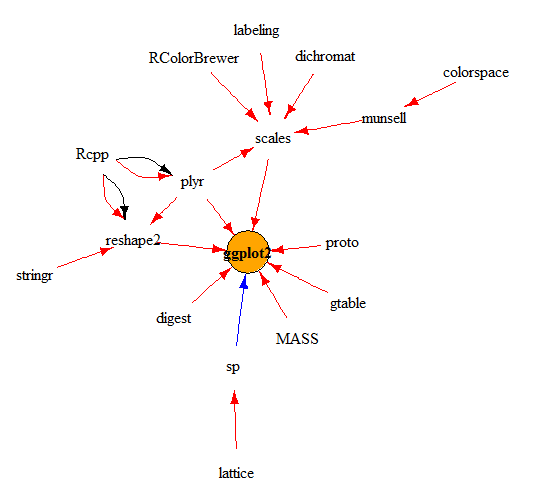
As you can clearly see from the above example, the package “ggplot2” has a import dependency on 22 packages and another 35 suggest packages. Let’s try to visualize how this dependency structure looks like. Here is a code which will help you with that :

plot(makeDepGraph(pkgs, includeBasePkgs=FALSE, suggests=FALSE, enhances=TRUE), 
 legendPosEdge = c(-1, 1), legendPosVertex = c(1, 1), vertex.size=20)

As we can clearly see, packages like “lattice” or “stringr” are not directly linked to ggplot2, but should be installed prior to installing ggplot2.

Hopefully, now we have gained decent knowledge on these packages, let’s do some practice problems on them for deeper understanding.

Practice Problems

Here are a few questions using which we will understand more about R packages :

1. Which packages forms the foundation of R? In other words, which packages are the most used or referred package in R?

2. How many package were added in the window Oct’14 to April ’15?

3. How has the importance of  most critical package changed over the window Oct’14 to April ’15? Has it increased, decreased or remained same?

4. What are the dependencies of the most critical package?

Solutions

1. Packages which form foundation of R :

We will use PageView algorithm to find the most important packages. The simple philosophy being, the packages which are referred by many different packages on R are the ones forming the foundation of R. Our analysis will be based on the latest CRAN image available. Here is the code which can help you to find the same:

# Major part of this code has been written by  Andrie de Vries

library(miniCRAN)
library(igraph)
library(magrittr)

#Use the latest image of CRAN to find dependencies

MRAN <- "http://mran.revolutionanalytics.com/snapshot/2015-04-01/"

pdb <- MRAN %>%
 contrib.url(type = "source") %>%
 available.packages(type="source", filters = NULL)

g <- pdb[, "Package"] %>%

 makeDepGraph(availPkgs = pdb, suggests=FALSE, enhances=TRUE, includeBasePkgs = FALSE)

# Use the page.rank algorithm

pr <- g %>%
 page.rank(directed = FALSE) %>%
 use_series("vector") %>%
 sort(decreasing = TRUE) %>%
 as.matrix %>%
 set_colnames("page.rank")

# Display results ---------------------------------------------------------

head(pr, 10)

                     page.rank
MASS                0.020425142
Rcpp                0.018934424
Matrix              0.009553795
lattice             0.008853670
mvtnorm             0.008597332
ggplot2             0.008207035
survival            0.008022737
plyr                0.006900871
igraph              0.004725656
sp                  0.004640548

As is clearly seen in the table above, the most important packages are “MASS” and “Rcpp”. Evidently, they form the backbone of R.

2. How many packages were added in Oct’14 – Apr’15

We’ll run a similar code to find the number of packages in Oct’14 and then make a comparison between them. Following is the code to solve this question:

MRAN <- "http://mran.revolutionanalytics.com/snapshot/2014-10-01/"

pdb1 <- MRAN %>%
 contrib.url(type = "source") %>%
 available.packages(type="source", filters = NULL)

g1 <- pdb1[, "Package"] %>%

makeDepGraph(availPkgs = pdb, suggests=FALSE, enhances=TRUE, includeBasePkgs = FALSE)

pr1 <- g %>%
 page.rank(directed = FALSE) %>%
 use_series("vector") %>%
 sort(decreasing = TRUE) %>%
 as.matrix %>%
 set_colnames("page.rank")

#Finally find the size of the two :

nrow(pr) - nrow(pr1)

[1] 498

498 packages were added in this duration. Wow, its like 70 packages every month!

3. How has this impacted the importance of the most critical package?

In section 1, we saw MASS as the most critical package with an importance of 0.020425142 in Apr’15. In case, if it proportionally goes up with lesser number of package in Oct’14, its importance can be calculated as:

~ 0.020425142 * nrow(pr)/nrow(pr1)   = 0.02212809

Now, let’s find its actual importance in Oct’14:

head(pr1, 1)

         page.rank
MASS     0.020854737

Hence, the importance of MASS has not dropped to the extent it should have because of the increase in the number of packages in the window.

This can be just because the new packages would have been using this package “MASS” equally and hence increasing the importance.

4 . What are the dependencies of the most critical packages?

This one is the simplest to crack. We already know the function which can bring out all the dependencies of a package. Following code will help you with this one :

pkgs <- "MASS"
pkgDep(pkgs, suggests=FALSE, enhances=FALSE, includeBasePkgs = TRUE)

 "MASS"      "grDevices" "graphics"  "stats"     "utils"

pkgDep(pkgs, suggests=TRUE, enhances=FALSE, includeBasePkgs = TRUE)

"MASS" "grDevices" "graphics" "stats" "utils" "grid" "lattice" "splines" "nlme" "nnet" "survival"

End Notes

PageRank comes very handy in any importance determining exercise which has a linkage structure to it. Similar analysis can be done on Python to understand the structure beneath the top level packages which we use so conveniently.  This analysis can also be done in social networks to understand the magnitude of influence a user has on social network.

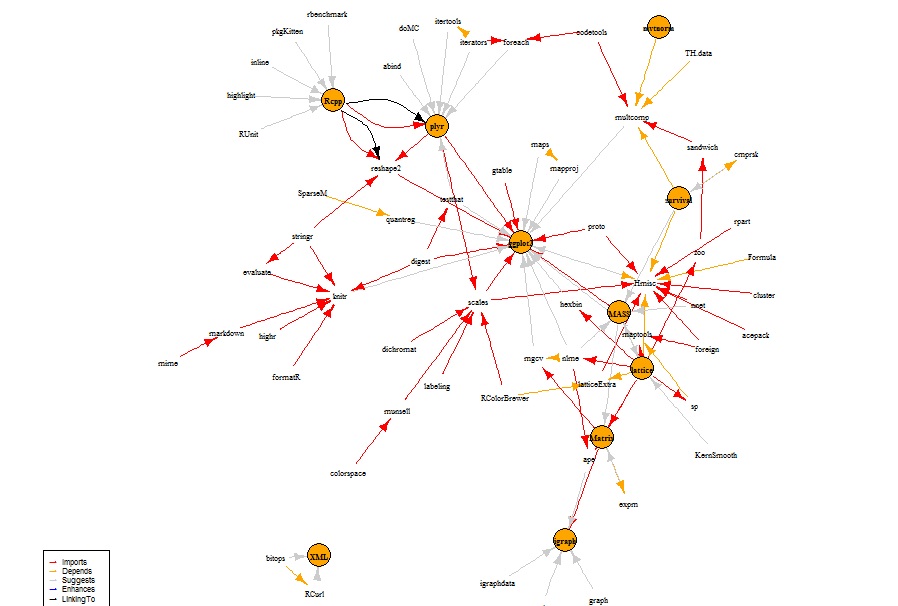
To end the discussion, let’s view the network structure of the top 10 packages on R :

Thinkpot: Can you think of more usage of Page Rank algorithm?  Share with us useful links to practice Page Rank algorithm in various fields.

Did you find this article useful? Do let us know your thoughts about this article in the box below.

If you like what you just read & want to continue your analytics learning, subscribe to our emails, follow us on twitter or like our facebook page.

Tavish Srivastava

Tavish Srivastava, co-founder and Chief Strategy Officer of Analytics Vidhya, is an IIT Madras graduate and a passionate data-science professional with 8+ years of diverse experience in markets including the US, India and Singapore, domains including Digital Acquisitions, Customer Servicing and Customer Management, and industry including Retail Banking, Credit Cards and Insurance. He is fascinated by the idea of artificial intelligence inspired by human intelligence and enjoys every discussion, theory or even movie related to this idea.