Introduction
Hi everyone! This is the 4th article of the series of data science interview questions. In case you want to revisit the previous ones, tap here. This article will cover all you need to know about boosting algorithms.
We have various Machine Learning algorithms to build predictive models. We choose the boosting algorithms based on our problem and prediction requirements. Although sometimes regular ML algorithms are not enough to get good results; hence we use an ensemble approach to build more robust and better-performing models. Ensemble methods combine the boosting algorithms in three different ways:
1.) Bagging
2.) Boosting
3.) Stacking
This article will discuss some boosting algorithms and the stacking ensemble method. Data scientists use these algorithms to win Kaggle competitions and real-world projects. To learn about Bagging, refer to my previous article here.
This article will discuss the Gradient Boosting family algorithms, including XGBoost and LightGBM. We will discuss these algorithms with their implementation in Python to solve the Crop Damage projection problem.
The dataset and problem statement are available on the Analytics Vidhya platform. The dataset contains information regarding the health of crops and soil. This problem is the multiclass classification problem denoting the soil damage condition, 0 being no damage and 2 being the most severe damage.
So first, let’s import, clean, and split the dataset using Python, Pandas, and Scikit-Learn.
import pandas as pd
import numpy as np
import matplotlib.pyplot as plt
import seaborn as sns
from sklearn.model_selection import train_test_split as tst
from sklearn.metrics import classification_report, confusion_matrix
from sklearn.ensemble import GradientBoostingClassifier
import xgboost
import lightgbm
train = pd.read_csv('train.csv')
X = train.drop(['ID','Crop_Damage'], axis=1)
y = train['Crop_Damage']
X.fillna(0, inplace = True)

x_train, x_val, y_train, y_val = tst(X, y, test_size=0.25, stratify = y)
Boosting Algorithms – Data Science Interview Questions
-
What is Gradient Boosting?
We use Gradient to calculate derivatives to minimize residual errors. The Gradient Boosting algorithm works for both classification and regression analysis.
Gradient Boosting tries to reduce the error from the predecessor decision tree. It creates a new tree to fit the residuals of the previous tree to improve the prediction of the weak learner. Let’s understand the working of Gradient Boosting:
- Train the weak learner
- The first iteration prediction is the average of all the target variable values.
- Then calculates residuals by subtracting the predicted value from the actual labels.
- Now it builds a tree to predict the residuals with minimum depth.
- Then it calculates the new prediction using the following formula: new_prediction= old_predition+learning_rate*residual
- It calculates the predicted value with the above process for all rows.
- Then it repeats the whole process until the residuals get minimized significantly.
- The final result is the output of the following equation:
Final_prediction = first_prediction+learning rate* first residual + learning rate * second residual, and so on.
Let’s use the Gradient Boosting classifier to solve our problem.
gbc = GradientBoostingClassifier()

gbc.fit(x_train, y_train)

pred = gbc.predict(x_val)

print(classification_report(y_val, pred))
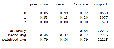
The overall accuracy with Gradient Boosting is 84%, but it cannot predict label 2; hence it is not a good performance.
2. Explain what XGBoost is?
The XGBoost (or Extreme Gradient Boosting) algorithm is a modified version of the Gradient Boosting algorithm. XGBoost (Extreme Gradient Boosting) is an open-source software library that provides a gradient boosting framework for C++, Java, Python, R, and Julia. It has become one of the most popular machine learning algorithms in recent years due to its efficiency, flexibility, and ease of use.
Since Gradient Boosting is a type of ensemble machine learning algorithm that combines the predictions of multiple weaker models to create a robust, more accurate model. XGBoost builds on this idea by using decision trees as the base models and a gradient descent algorithm to improve the model’s predictive performance.
One of the critical features of XGBoost is its ability to handle missing values and imbalanced data. It also performs regularization, which can prevent overfitting. Additionally, XGBoost is fast and scalable, making it a good choice for large-scale and high-dimensional data.
Overall, XGBoost is a powerful and widely-used machine learning algorithm that we can apply to various problems. It often gets used in competitions and hackathons on Kaggle and other platforms, where it has consistently been among the top-performing algorithms.
xgb = xgboost.XGBClassifier()

xgb.fit(x_train, y_train)

predics = xgb.predict(x_val)

print(classification_report(y_val, predics))
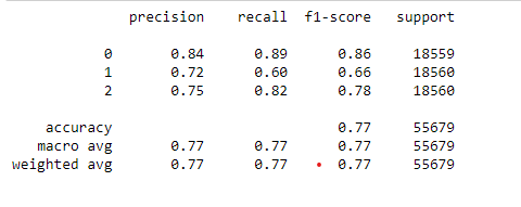
XGBoost is giving fine results with 77% accuracy, but we expected better from this algorithm.
3. What is LightGBM Algorithm?
LightGBM (Light Gradient Boosting Machine) is a gradient boosting framework that uses tree-based algorithms and follows the principle of leaf-wise growth, as opposed to depth-wise growth.
Like XGBoost, LightGBM is an ensemble learning algorithm that combines the predictions of multiple weak models to create a robust and more accurate model. The main difference between the two is that LightGBM uses a leaf-wise tree growth algorithm, which tends to converge faster than the depth-wise algorithm used by XGBoost. This approach makes LightGBM faster and more efficient, especially on large-scale data.
Another critical feature of LightGBM is that it supports both continuous and categorical features, allowing it to be applied to a wide range of problems. It also has built-in support for parallel and GPU training, making it even faster and more scalable than XGBoost.
LightGBM is a powerful and efficient gradient-boosting library well-suited for large-scale and high-dimensional data. It has become a popular choice among data scientists and machine learning practitioners due to its speed and performance.
params = {}

params['learning_rate'] = 0.04

params['max_depth'] = 18

params['n_estimators'] = 3000

params['objective'] = 'multiclass'

params['boosting_type'] = 'gbdt'

params['subsample'] = 0.7

params['random_state'] = 42

params['colsample_bytree']=0.7

params['min_data_in_leaf'] = 55

params['reg_alpha'] = 1.7

params['reg_lambda'] = 1.11

params['class_weight']: {0: 0.44, 1: 0.4, 2: 0.37}

clf = lightgbm.LGBMClassifier(**params)

clf.fit(x_train, y_train)

preds = clf.predict(x_val)

print(classification_report(y_val, preds))
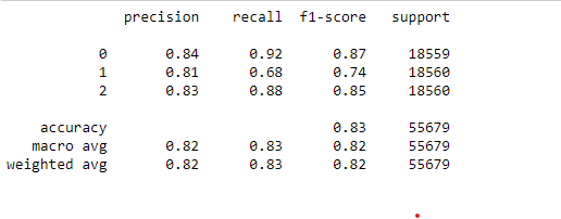
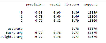
LightGBM classifier outperformed the XGBoost and Gradient Boosting with 83% accuracy overall and more than 0.7 F1-Score for each label.
4. What is CatBoost Algorithm?
CatBoost is an open-source gradient-boosting library designed to work with categorical data.
One of the main advantages of CatBoost is that it can automatically handle categorical variables without any preprocessing, which is a common problem in machine learning. This algorithm is suitable for working with datasets with multiple categorical features.
CatBoost also uses a novel gradient boosting algorithm called Ordered Boosting. It is specifically designed to handle categorical features. This algorithm uses decision trees as the base model and applies the gradient descent algorithm to improve the model’s predictive performance.
In addition to its ability to handle categorical data, CatBoost supports regularization, preventing overfitting and improving the model’s generalizability. It also has built-in parallel and GPU training support, making it fast and scalable.
Overall, CatBoost is a powerful and effective gradient-boosting library that is well-suited for working with categorical data. It has become a popular choice among data scientists and machine learning practitioners for its speed and performance.
from catboost import CatBoostClassifier
cbc = CatBoostClassifier()

cbc.fit(x_train, y_train)

cbc_pred = cbc.predict(x_val)

print(classification_report(y_val, cbc_pred))
The CatBoost gives us a 78% accuracy score, which is pretty good.
5. What is Stacking Algorithm?
Stacking is an ensemble learning technique that combines multiple machine learning models to create a stronger, more accurate model. It is called “stacking” because the individual models are “stacked” to form a single, unified model.
The idea behind stacking is to train a set of base models on the original training data, then use these base models to make predictions on a new, hold-out dataset. These predictions are then used as features for a higher-level model, which is trained to make the final predictions. This higher-level model, known as the meta-model, is trained to take into account the strengths and weaknesses of the individual base models and make a more accurate prediction.
One of the key benefits of stacking is that it can improve the performance of the individual base models by allowing them to learn from each other. This is because the meta-model can combine the predictions of the base models in a way that considers their different strengths and weaknesses.
Overall, stacking is a powerful ensemble learning technique that can be used to improve the performance of machine learning models. It is instrumental in situations where the base models have different types of errors or strengths, allowing them to learn from each other and produce more accurate predictions.
from sklearn.ensemble import StackingClassifier

from sklearn.linear_model import LogisticRegression

from sklearn.neighbors import KNeighborsClassifier

from sklearn.naive_bayes import GaussianNB

from sklearn.tree import DecisionTreeClassifier

# dtc = DecisionTreeClassifier() # initialising KNeighbors Classifier

# NB = GaussianNB() # initialising Naive Bayes

estimators = [

('dtc', DecisionTreeClassifier(random_state=42)),

('NB', GaussianNB())]

lr = LogisticRegression() # defining meta-classifier

clf_stack = StackingClassifier(estimators =estimators, final_estimator = lr)

clf_stack.fit(x_train, y_train)

stack_pred = clf_stack.predict(x_val)

print(classification_report(y_val, stack_pred))
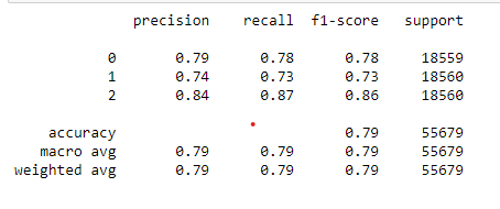
The stacking approach gives good results with 79% accuracy and seems to be the second best after LightGBM.
6. What is Blending Ensemble Approach?
Blending is an ensemble learning technique similar to stacking but with one key difference. In blending, the predictions of the base models are not used as features for a higher-level model. Instead, the predictions of the base models are combined using a simple average or weighted average to produce the final prediction.
The main advantage of blending over stacking is that it is simpler and faster to train. Because no meta-model needs to be trained, blending can be done in a single step, whereas stacking requires training the base models and the meta-model separately.
However, the simplicity of blending also means that it is less flexible and may not be as accurate as stacking in some situations. Because there is no meta-model to learn from the base models, blending cannot consider the strengths and weaknesses of the individual base models. As a result, it may not be as effective at improving the performance of the base models.
Overall, blending is a simple and fast ensemble learning technique that can be used to combine the predictions of multiple machine learning models. It is a good choice when speed and simplicity are important, but it may not be as effective as other ensemble methods in some cases.
# get a list of base models

def get_models():

models = list()

models.append(('lr', LogisticRegression()))

models.append(('knn', KNeighborsClassifier()))

models.append(('cart', DecisionTreeClassifier()))

# models.append(('svm', SVC()))

models.append(('bayes', GaussianNB()))

return models


# fit the blending ensemble

def fit_ensemble(models, X_train, X_val, y_train, y_val):

meta_X = list()

for name, model in models:

model.fit(X_train, y_train)

# predict on hold out set

yhat = model.predict(X_val)

# reshape predictions into a matrix with one column

yhat = yhat.reshape(len(yhat), 1)

# store predictions as input for blending

meta_X.append(yhat)

# create 2d array from predictions, each set is an input feature

meta_X = np.hstack(meta_X)

# define blending model

blender = LogisticRegression()

# fit on predictions from base models

blender.fit(meta_X, y_val)

return blender


# make a prediction with the blending ensemble

def predict_ensemble(models, blender, X_test):

meta_X = list()

for name, model in models:

# predict with base model

yhat = model.predict(X_test)

# reshape predictions into a matrix with one column

yhat = yhat.reshape(len(yhat), 1)

# store prediction

meta_X.append(yhat)

# create 2d array from predictions, each set is an input feature

meta_X = np.hstack(meta_X)

# predict

return blender.predict(meta_X)


# create the base models

models = get_models()

# train the blending ensemble

blender = fit_ensemble(models, x_train, x_val, y_train, y_val)

# make predictions on test set

yhat = predict_ensemble(models, blender, x_val)

print(classification_report(y_val, yhat))
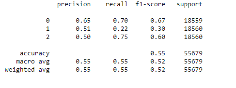
The blending algorithm performed below expectations and gave only 55% overall accuracy.
7. What is AdaBoost?
The AdaBoost or Adaptive Boosting ensemble learning algorithm is one of the first boosting algorithms ever accepted by Data Science. Yoav Freund and Robert Schapire proposed the Adaboost algorithm in 1996 for the first time.
AdaBoost (Adaptive Boosting) is a type of ensemble learning algorithm that is used to improve the performance of a base learning algorithm. It combines multiple weaker models, called “weak learners,” to create a more accurate and robust model. In other words, this algorithm accumulates multiple classifiers into one model to boost the model’s performance. It is an iterative ensemble approach that assigns more weight to weak learners and retrains them iteratively.
The key idea behind AdaBoost is to train the weak learners sequentially, with each learner focusing on the mistakes made by the previous learner. This algorithm allows the weak learners to “adapt” to the previous learners’ mistakes and improve the model’s overall performance.
AdaBoost is an iterative algorithm that repeats the training process multiple times, adding a new weak learner to the model each time. The algorithm assigns higher weights to the previously misclassified instances at each iteration. So that the new learner will focus on those instances and try to classify them correctly. One of the main advantages of AdaBoost is that it is a fast and simple algorithm that is easy to implement and understand. It is versatile and can be used with various base learning algorithms, such as decision trees or support vector machines. Overall, AdaBoost is a powerful and widely-used ensemble learning algorithm that can improve the performance of a base learning algorithm. It is often used in various applications, including image and video recognition, natural language processing, and medical diagnosis.
from sklearn.ensemble import AdaBoostClassifier

abc = AdaBoostClassifier()

abc.fit(x_train,y_train)

abc_pred = abc.predict(x_val)

print(classification_report(y_val, abc_pred))
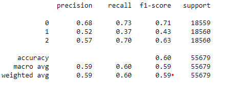
The Adaboost model gives us only 60% accuracy, which is less than we got earlier with other models.
So we have a winner among all boosting algorithms for our problem as LightGBM Classifier with overall 83% accuracy. We can improve the performance with feature engineering, data preprocessing, and hyperparameter tuning. We will leave this part for the future scope of this article.
Conclusion
We have discussed all the boosting algorithms, such as Gradient Boosting, XGBoost, CatBoost, Stacking, Blending, LightGBMBoost, and AdaBoost. Now let us summarize the article using the following key takeaways:
- Gradient Boosting is an ensemble learning algorithm that combines the predictions of multiple weaker models to create a robust and more accurate model.
- XGBoost is a gradient boosting algorithm that uses decision trees as the base models and a gradient descent algorithm to improve the model’s predictive performance. It is especially effective at handling missing values and imbalanced data and is fast and scalable, making it a popular choice for large-scale and high-dimensional data.
- LiGhtGBMBoost is a gradient-boosting framework that uses tree-based algorithms and follows the principle of leaf-wise growth. It is designed to be faster and more efficient than other gradient-boosting libraries, especially on large-scale data. It supports continuous and categorical features and built-in support for parallel and GPU training.
- CatBoost can automatically handle categorical variables without any preprocessing and uses a novel gradient boosting algorithm called Ordered Boosting to handle categorical features effectively. It also supports regularization and has built-in support for parallel and GPU training.
- Stacking trains a set of base models on the original training data and then uses these base models to make predictions on a new, hold-out dataset. These predictions are used as features for a higher-level model, which is trained to make the final predictions. This allows the base models to learn from each other and improve the model’s overall performance.
- Blending combines the predictions of multiple machine learning models using a simple average or weighted average.
- AdaBoost trains multiple weak learners sequentially, with each learner focusing on the mistakes made by the previous learner. This allows the weak learners to “adapt” to the previous learners’ mistakes and improve the model’s overall performance. It is a fast and simple algorithm that is easy to implement and versatile and can be used with various base learning algorithms.
Ready to master boosting algorithms? Join our course and gain hands-on experience in leveraging these powerful techniques to enhance your models’ performance—unlock your potential today!
