Introduction
Many different datasets are available for data scientists, machine learning engineers, and data engineers. Small datasets that easily fit in your computer’s RAM, medium-sized datasets that barely fit on your computer’s storage, and large datasets that look hard to handle are all examples of dataset sizes. Finding the best tools to evaluate each dataset can be difficult because they all have different problems and restrictions. Dask is the best option for optimum performance and quick calculation of medium to large datasets. Let’s start understanding Dask, its significance, functioning, and much more in this article.
Learning Objectives
- Understanding Dask and its significance compared to other libraries.
- Understanding the functioning of Dask.
- Acquire knowledge of the various Dask Interfaces.
- Hands-on experience in implementing a machine learning project using Dask.
This article was published as a part of the Data Science Blogathon.
Table of Contents
- Why Dask?
- How Dask Works?
- Configure your system
- Introducing Dask
- Dask Interfaces
-
Dask High-level APIs
-
Dask Low-Level APIs
- Working on a dataset
- Conclusion
Why Dask?
Pandas and NumPy are great libraries, but when it comes to large datasets, they are inefficient because they take longer to compute than smaller datasets. This is where Dask comes in. The first step to understanding Dask is to know one of the key features that sets Dask apart from the competition is that it is entirely written and implemented in Python. The collection APIs of Dask is designed to scale NumPy, pandas, and scikit-learn natively. It uses parallel and distributed computing to overcome the limits of a single machine.

Source: https://tutorial.dask.org/
How Dask Works?
To understand how Dask works let’s go through an example; let’s say I am cooking biryani for my roommates. It is easy for me to handle. But preparing many servings for a busy dinner service in my town would present a significant challenge. It’s time to seek help!
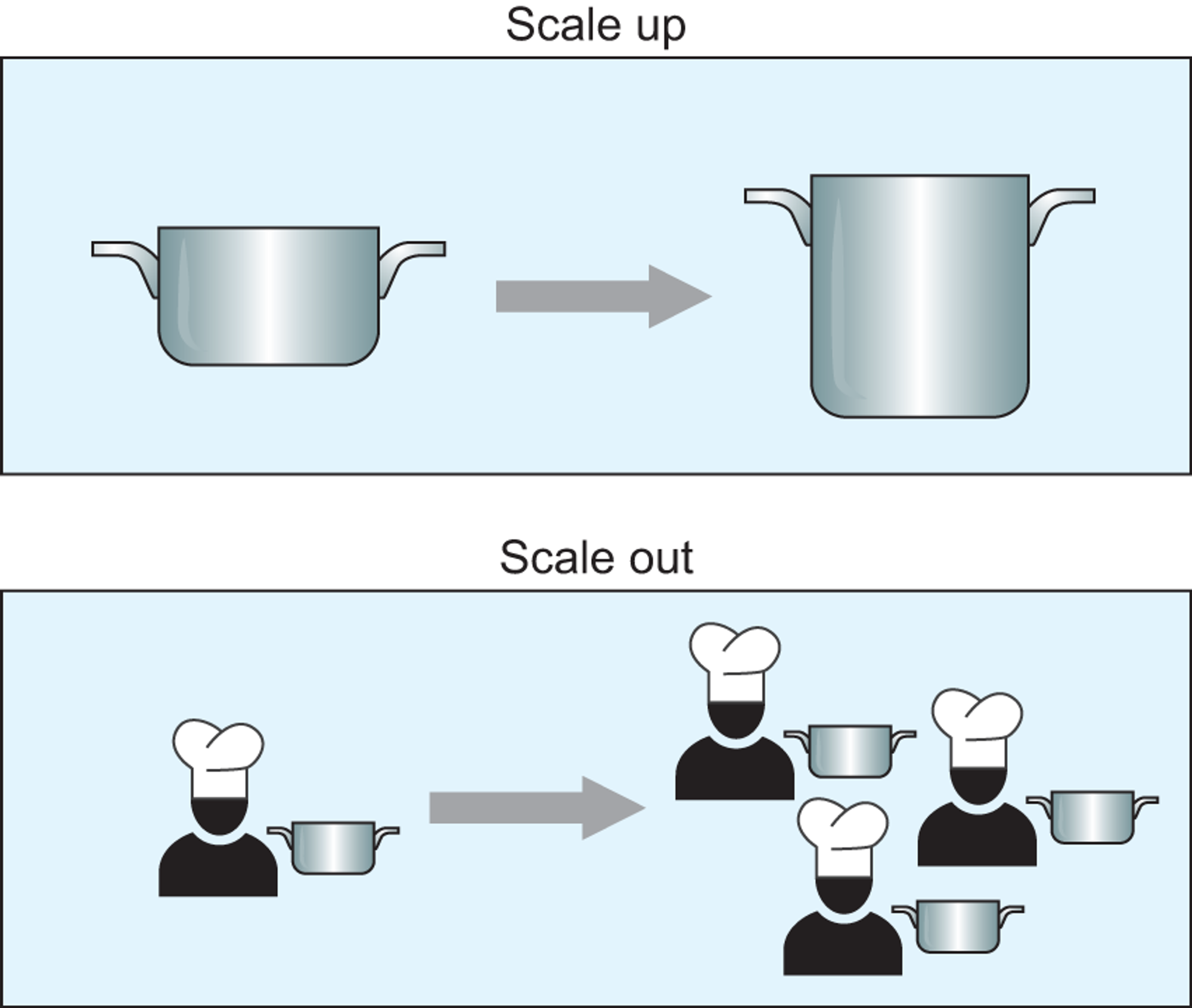
First, I must decide how to handle the resource problem: should I advance my kitchen equipment to be more efficient, or should I hire more cooks to help share the workload? In computing, these two approaches are called scaling up and scaling out, respectively.

Source: https://tutorial.dask.org/
Scaling out can be the better option to take advantage of parallelism while working with large datasets. To help share the workload, I hire 9 additional cooks. All 10 of us focusing 100% of our attention and time on the process can reduce five hours of work to 30 minutes, assuming equal skill levels.
Introducing Dask
Dask was launched in late 2014 by Matthew Rocklin, to bring native scalability to the Python Open Data Science Stack and overcome its single-machine restrictions. Dask breaks large computations into smaller, more manageable tasks that can be executed in parallel. These tasks are then executed by a scheduler responsible for managing the tasks to be executed and the data distribution between them.
The scheduler uses a task graph to represent the dependencies between tasks, which allows it to execute tasks in the most efficient order possible. The user creates the task graph when they define their computation using Dask’s high-level APIs, such as Dask Array, Dask Dataframe, and Dask Delayed. It allows for parallel computing on larger-than-memory datasets by breaking them into smaller chunks, called blocks, and only loading and processing one block at a time. This allows Dask to process datasets that are too large to fit into memory by using disk storage.
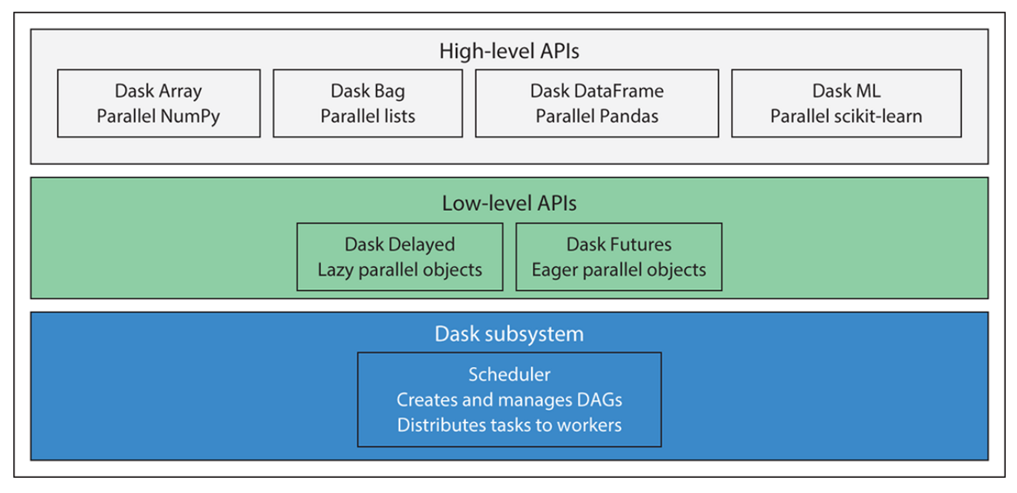
Dask uses multi-threading and multi-processing to take advantage of multiple cores and CPUs available in a single machine. This allows Dask to perform parallel computation even on a single machine. Dask consists of several different components and APIs, which can be categorized into three layers: the scheduler, low-level APIs, and high-level APIs. An overview of these components can be seen in the fig below.

The computations are represented in the code by two different types of objects: dask delayed objects and dask futures objects. Task scheduling coordinates and keeps track of computations on separate CPU cores. The dask delayed evaluates later, whereas the dask futures assess instantly, which is the main distinction between the two.
Configure your System with Dask
Let’s configure our system and take a look at the Dask functionalities. To do so, install Anaconda and, once installed, enter the following code into your Anaconda Prompt.
conda install dask
Now that we have installed Dask on our system let’s look at the Dask functionalities.
Dask Interfaces
Dask has several high-level and low-level APIs or collections.
The high-level APIs are
- Dask Dataframe
- Dask Array
- Dask Bag
- Dask ML
The Low -level APIs are
- Dask Delayed
- Dask Futures
Dask High-level APIs or Collections
1. Dask Dataframe
Parallel to Pandas Dataframe is Dask Dataframe. Along the index, it divides the data into smaller, chunked dataframes. The processing is carried out in an organized parallel fashion across several processors.
Here is a sample code for using Dask Dataframe.
import dask.dataframe as dd
import pandas as pd
#reading  a CSV file using pandas
df = pd.read_csv('epl_soccer_data.csv')
#converting pandas dataframe to Dask dataframe and splitting into 4 partitions
dask_df = dd.from_pandas(df, npartitions=4)
# to display columns in the dataframe
dask_df.columns
# using groupby() method to group one or more columns
# compute() method computes the result and returns a pandas dataframe
dask_df.groupby('Club').mean().compute()
#filtering
dask_df.query("Goals > 10").compute()
#value count of a particular column
dask_df.Club.value_counts().compute() #no of players in each club
#Pearson's correlation
dask_df[['Goals','DistanceCovered(InKms)']].corr().compute()
2. Dask Array
Numpy arrays and Dask arrays are comparable. It is made out of the Numpy ndarray subset. It offers chunked parallel arrays that can be processed sequentially across one or more processors.
Here is a sample code for using Dask Array.
#import dask array and numpy
import dask.array as da
import numpy as np
# creates an array of 1000 x 1000 using numpy
x = np.random.rand(1000, 1000)
#converting numpy array into dask array with chunk size 100x100
dask_x = da.from_array(x, chunks=(100, 100))
#summing all the values in the array
dask_x.sum().compute()
#dot product of two arrays
y = np.random.rand(1000, 1000)
dask_y = da.from_array(y, chunks=(100, 100))
dot_product = da.dot(dask_x, dask_y).compute()
#concatenation of two arrays
da.concatenate([dask_x,dask_y], axis =0).compute()
3. Dask Bag
A versatile parallel collection for handling big data sets is called a Dask bag. It analyzes unstructured data like text, JSON, or log files and is comparable to a Python list. Here is a sample code for using Dask Bag.
import dask.bag as db
#creating a bag from an existing python iterable
data = range(1000)
dask_bag = db.from_sequence(data, npartitions=2)
#load data directly from text files
bag = db.read_text('myfile.txt')
#map
squared_data = dask_bag.map(lambda x: x ** 2).compute()
#filter
filtered_data = dask_bag.filter(lambda x: x % 2 == 0).compute()
4. Dask ML
A parallel implementation of scikit-Learn, is Dask ML. This library allows the use of Dask in machine-learning workflows. Scalable machine learning methods, model selection, and evaluation tools are provided.
To install Dask-ml in Anaconda, enter the following code into your Anaconda Prompt.
conda install -c conda-forge dask-ml
We build a regression model using Dask-ml in the working-on-a-dataset section. There we can see the various tools of Dask-ml.
Dask Low-Level APIs
1. Dask Delayed
The Dask delayed function decorates your functions so that they operate lazily. You can describe a task as a function call using dask.delayed, and Dask will create a task graph that can be executed later. Dask can optimize the execution and reduce the amount of computation required by delaying task execution until the result is required.
In this example code, the function add is decorated with dask.delayed, and a delayed object is returned instead of the result of the function. Before calling compute(), the computation is not carried out.
import dask
@dask.delayed
def add(a, b):
    return a + b
x = add(1, 2)
x # object is returned instead of the result of a function
#To get the result we have to use compute()
result = x.compute()
print(result)  # 3
2. Dask Futures
Most of the python futures API has been reimplemented in Dask Futures, allowing you to expand your python futures process over a Dask cluster with very little code modification. Similar to dask.delayed, this interface is useful for arbitrary task scheduling. Still, it is instantaneous rather than lazy, giving it more flexibility in scenarios where the calculations may change over time. Here is the code to understand Dask Futures.
# creating a function
def inc(x):
    return x + 1
def add(x, y):
    return x + y
# Submit function returns a Future, which refers to a remote result.
a = client.submit(inc, 10)  # calls inc(10) in background thread or process
b = client.submit(inc, 20)  # calls inc(20) in a background thread or process
a #Future: status: finished, type: int, key: inc-b8aaf
a.result()  #data arrives from the remote
Working on a Dataset
To put what we have learned into practice. Let’s attempt to use Dask to create a regression model using the EPL soccer dataset. You can download the dataset from here.
# Importing necessary dependencies
import os
import math
import dask
import dask.dataframe as dd
from dask.distributed import Client
import numpy as np
import pandas as pd
import dask_ml
#check the file('epl_soccer_data.csv') in the list of filenames in a directory
os.listdir()
#size of the file in GB
size = os.path.getsize('epl_soccer_data.csv')/math.pow(1024,3)
print("size in GB : {}".format(size))
# Client instance can be used to submit tasks to a Dask scheduler and monitor their progress.
# 4 worker processes will be started.
# Each worker process will have 1 thread.
# Each worker process is limited to 2GB of memory.
client = Client(n_workers =4, threads_per_worker =1, memory_limit ='2GB')
client
# Reading the data
ddf = dd.read_csv('epl_soccer_data.csv', assume_missing = True)
# returns first n rows of a dataframe
ddf.head()
# Data cleaning, checking for null values
ddf.isna().sum().compute() #zero null values found
# droping the duplicates
ddf.drop_duplicates()
ddf= ddf.drop('PlayerName', axis =1)
# Declaring the categorical variable column
ddf = ddf.categorize(columns=['Club'])
# Data preprocessing, encoding the categorical variable club column
from dask_ml import preprocessing
de = preprocessing.DummyEncoder()
ddf= de.fit_transform(ddf)
ddf.head(10)                     # Shows the table (After encoding the categorical variable)
#checks the data types of columns
ddf.dtypes
# Declaring the Dependent and independent variables
#declaring the dependent variable
y=ddf.Score
#declaring independent variables
X=ddf.drop(columns=['Score'])
#converting into Arrays
X =X.to_dask_array(lengths=True)
y = y.to_dask_array(lengths = True)
# Splitting the data into training and testing
from dask_ml.model_selection import train_test_split
X_train, X_test, y_train, y_test = train_test_split(X,y, test_size = 0.3)
# Fitting a linear regression model
from dask_ml.linear_model import LinearRegression
lr = LinearRegression(solver ='lbfgs',max_iter =200)
lr_model = lr.fit(X_train, y_train)
# Model results
#Coefficents of the X variables
lr_model.coef_
# y predicted values
y_predicted = lr_model.predict(X_test)
# Here we are importing the metrics.
# To know the performance of the regression model we find various metrics of the model.
from dask_ml.metrics import mean_squared_error, r2_score
from math import sqrt
r2_score(y_test, y_predicted)               # Gives the r2_score value of the predicted model
sqrt(mean_squared_error(y_test, y_predicted))
mean_squared_error(y_test, y_predicted)
Conclusion
In conclusion, Dask is a powerful library that provides parallel and distributed computing capabilities for large-scale data processing. With its various interfaces and compatibility with popular data science tools, Dask offers a convenient and efficient solution for working with big data. This comprehensive guide has covered the basics of understanding Dask, including its importance, how it works, and its interfaces. By the end of this guide, readers should have a strong understanding Dask and its capabilities, as well as the knowledge and skills to implement a machine-learning project using Dask. As the demand for big data processing continues to grow, the importance of tools like Dask will only increase, making it a valuable asset for anyone in the data science field.
Key Takeaways
- Understanding Dask and its importance.
- Understanding Dask functioning and how it works.
- Familiarizing with Dask Interfaces and their functions.
- Building a regression model using Dask.
The media shown in this article is not owned by Analytics Vidhya and is used at the Author’s discretion.


Thanks a lot Prem for explaining Dask basics.. nice read!