Introduction
In the previous article, we understood the complete flow of the decision tree algorithm. In this article, let‘s understand why we need to learn about the random forest. when we already have a decision tree algorithm. Why do we need Random forest? What is it all about? Similar to the decision tree. Random Forest is also a supervised machine-learning algorithm. It is extensively used in classification and regression. But, the decision tree has an overfitting problem.
Wondering what overfitting is? Overfitting occurs when the model is too complex and fits the data too closely. This means that the model is not able to make accurate predictions on unseen data. The Random Forest algorithm can address this issue by creating multiple Decision Trees, and combining their predictions to come up with more accurate predictions.
Learning Objectives
- Understanding the basics of ensembled learning.
- Familiarizing with the basics of Random forest.
- Understanding the importance of each step involved while building the complete random forest.
- Practical implementation of the random forest using python.
- Understanding how the overfitting problem will be solved.
- We will also Understand how they can improve robustness.
This article was published as a part of the Data Science Blogathon.
Table of Contents
- Ensemble Techniques: What they are and how they work
- It is possible to understand how random forests work by following four simple steps?
-
Step 1: How a complete training Dataset is Used to build multiple trees?
-
Step 2: Multiple decision trees can be built by following steps
-
Step 3: Using multi-tree models for predicting the outcome, what is the process of expecting the result?
-
Step 4: When a model finalizes a result for regression or classification, what do we call this step ?
-
Conclusion
Ensemble Techniques: What They Are and How They Work?
In a decision tree, we have only one tree to answer the question. Let’s say we want to buy a phone. The following decision tree can be used to decide whether we should buy an iPhone or an Android phone.
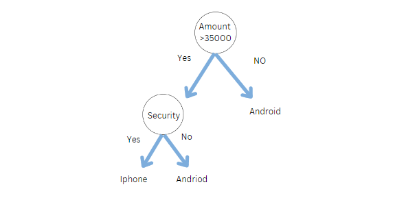
However, in real life, do we do the same thing, do we just ask one person to buy a phone? Definitely No. We ask multiple people like family, friends, experts, and salespersons.
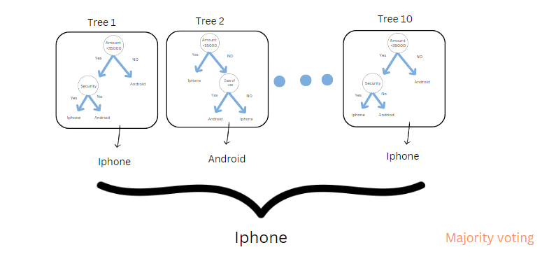
Assume each tree is like each person. So, if you ask 10 people (8 people said iPhone, and 2 people said Android. In Random forest classification, the final output is based on majority voting. We will buy an iPhone.
Note: what if we are building a regression model? We use mean or average.
We call the process of combing the several decision tree models a random forest. But, The question is, can we combine multiple models, like logistic, naïve Bayes, and KNN, and if yes, what do we call it? We call it Bagging and Boosting. They are two ensemble methods used in machine learning to improve the performance of a single model by combining the predictions of multiple models.
Bagging: bagging is a way of combing multiple models; it may be any model, as we discussed above, like knn, naive Bayes, logistic, etc. However, the result will be the same because the data input will be the same for all the models. To handle that, we will use a bootstrap aggregator.
- For example, if we have 10 models, each model trains on a different subset of the training data.
- The final prediction is usually the average or the majority vote of the predictions from all the models.
In addition to that, Bagging also reduces variance because of the two points above.
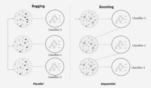
Boosting: Conversely, BOOSTING produces strong learners by combining weak ones. In the above image, you can see that it is following sequential training.
Types of Boosting algorithms
1. Adaboosting
2. Gradient boosting
3. XGboost
We will cover all of these topics in the upcoming articles
Step-wise Procedure to Understand How Random Forest Works
Yes, it’s possible to understand the working of the random forest in 4 simple steps. But, before that, we need to understand one question about Random Forest.
Which type of ensembled learning random forest belongs to?
It belongs to bagging, where we build multiple decision trees called random forest.
Understanding random forests require a step-by-step approach. Here is a step-by-step guide.
Step 1: How a Complete Training Dataset is Used to Build Multiple Trees?
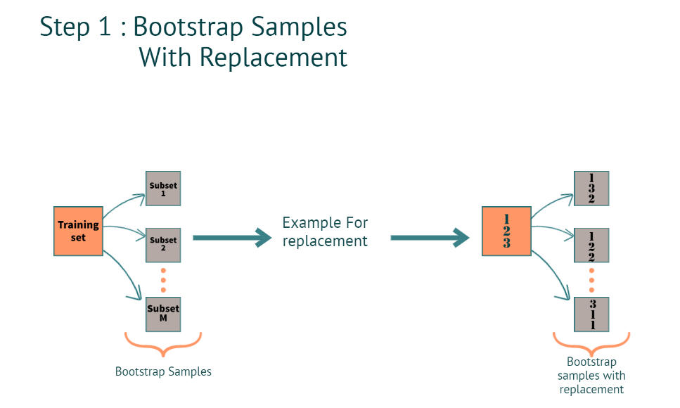
When we have a training dataset. The model creates a bootstrap sample with the replacement.
What is Bootstrap?
Creating multiple subsets from the actual training dataset.
How do we create multiple subsets when we have Rows and columns in the training dataset? and what is with replacement?
Rows:
When we say with thereplacement(refer to the image below for better understanding), in a subset, we can have the same row multiple times. as you can see in subset 2, the 2nd row is repeated 2 times, and in subset 3 1st row is repeated 2 times.
Columns:
1. For classification, it’s a square root of the total number of features
Example: let’s say we have a total of 4 features for each subset we will have
The square root of 4= 2. which is 2 features for each tree.
2. Regression: total number of features and dividing them by 3
Step 2: Multiple Decision Trees can be Built by Following Steps
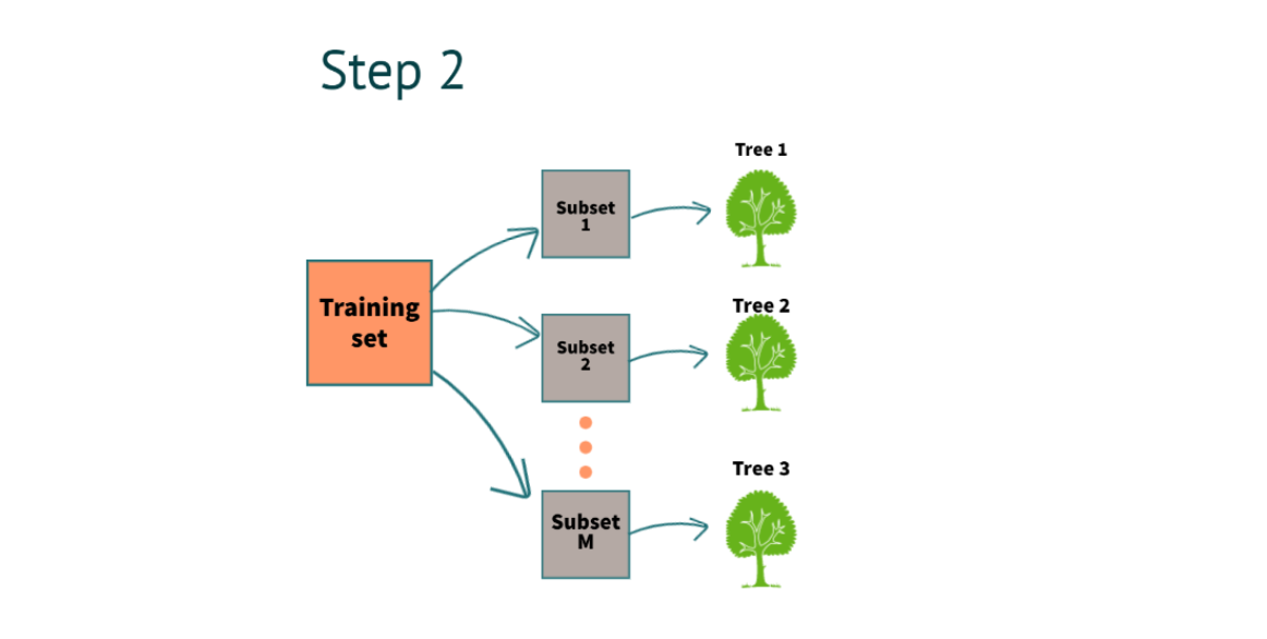
After completing step 1, we will build a decision tree for each subset. In the above example, we have 3 decision trees.
How were we able to build the decision trees from scratch?
To build a decision tree, we have to use two methods.
1. Gini
2. Entropy and Information gain
For a detailed understanding of math, you can refer to my Decision tree article in Analytics Vidhya.
Step 3: Using Multi-tree Models for Predicting the Outcome, What is the Process of Predicting the Result?
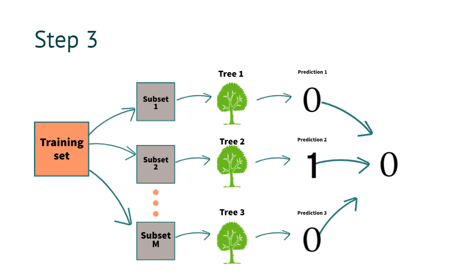
After building the decision tree now, it’s time to get the results. suppose we have new information for prediction
| salary | property | loan approval |
| 10k | No | ? |
The model predicts it as “0”. By combing all decision tree predictions above, as you can see in the image
What do we mean by combining the prediction of all the trees?
To understand it, we go to step four.
Step 4: When a Model Finalizes a Result for Regression or Classification, What is it Called?
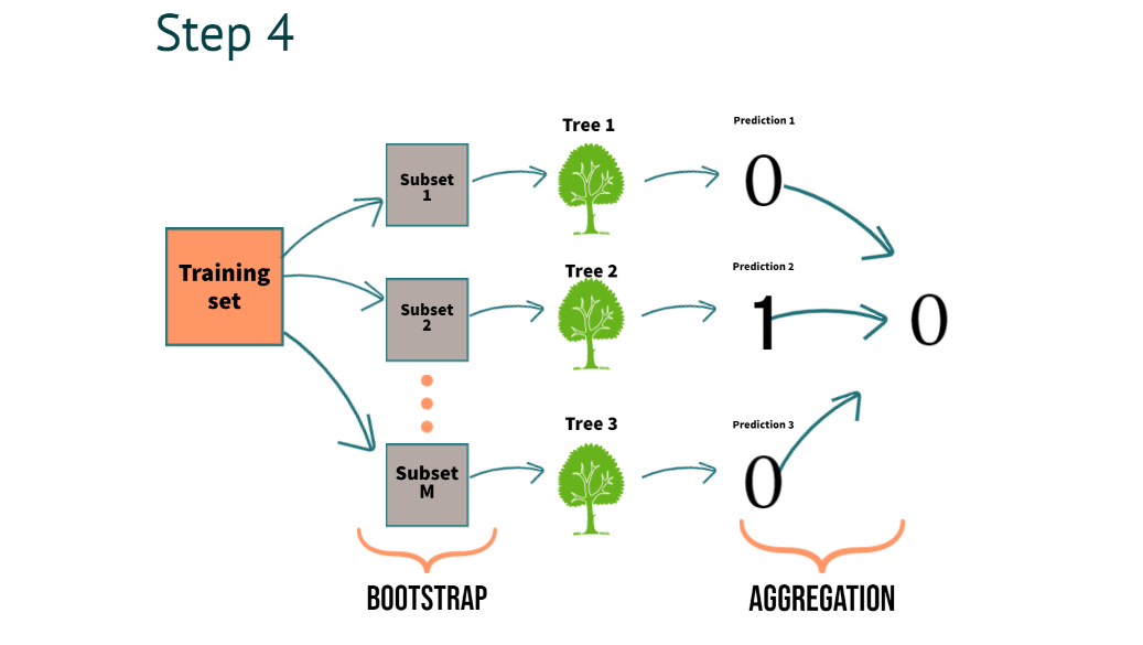
In Step 4, we can clearly understand the process of combining the predictions of multiple trees we call aggregation
- For classification, we use majority voting
- For regression, we use averaging
with this, we understand what exactly a bootstrap aggregation is all about.
Now, We need to understand how it benefits.
It reduces the variance. This helps build robust models, which work well even on unseen data.
Python Implementation
# Importing the necessary libraries
import pandas as pd
import numpy as np
from sklearn.datasets import load_iris
data = load_iris()
load the iris dataset from the sklearn library
# Convert the iris data into a Pandas data frame with feature names as column names
df = pd.DataFrame(data.data, columns=data.feature_names)
# Add a new column 'target' to the dataframe using target names and target codes
df['target'] = pd.Categorical.from_codes(data.target, data.target_names)
# Print first 5 rows of the dataframe
print(df.head())
We’re printing the first 5 rows after converting the data into a data frame.
# Split the data X and y
X = df.drop('target',axis=1)
y = df['target']
# Import train_test_split function from sklearn
from sklearn.model_selection import train_test_split
X_train, X_test, y_train, y_test = train_test_split(X, y, test_size=0.3, random_state=0)
# Import the RandomForestClassifier from sklearn
from sklearn.ensemble import RandomForestClassifier
classifier_rf = RandomForestClassifier(random_state=42, n_jobs=-1, n_estimators=20)
- Random_state(it helps to generate the same results every we run the model)
- n_jobs ( it uses all the processors)
- n_estimators( we are using 20 decision tree in the random forest. if we want, we can tune it.
# Fit the training data
classifier_rf.fit(X_train, y_train)
# Predict on testing data
y_pred = classifier_rf.predict(X_test)

from sklearn.metrics import confusion_matrix, classification_report, accuracy_score
print(confusion_matrix(y_test, y_pred))
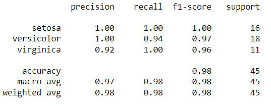
print(classification_report(y_test, y_pred))
We have the predictions saved in the y_pred variable. We can compare the actual vs. predicted using the report below.
Conclusion
In this article, we looked at the most popular algorithm. To summarize, we learned about Random Forest in detail. Let’s take a look at the key takeaways.
Key takeaways:
- Random forest gives us better accuracy than the single decision tree because the information will be passed to multiple trees.
- In real-time, we don’t get balanced datasets, and because of that, most of the machine learning models will be biased toward one specific class. Still, Random forest can handle an imbalanced dataset by randomizing the data.
- We use multiple decision trees to average the missing information. So, with Random forest, we can also handle the missing values.
- Lastly, It helps to build robust models in real-time by reducing variance.
Did you enjoy my article? Please comment below.
The media shown in this article is not owned by Analytics Vidhya and is used at the Author’s discretion.


