Introduction
Microsoft Excel is among the best programs for organizing and evaluating data. One of its most important features is the capacity to freeze panes. This function allows you to select certain rows or columns to keep visible while browsing the rest of your spreadsheet, making data monitoring and comparison easier. This post will look at using Excel’s Freeze Panes feature and provide some helpful tips and examples.

Overview
- Freezing panes in Excel keep specific rows or columns visible while scrolling through large datasets, aiding in data monitoring and comparison.
- Enhances navigation, maintains header visibility, and simplifies data comparison within extensive spreadsheets.
- Instructions for freezing the top row, first column, or multiple rows/columns using the View tab and Freeze Panes option.
- Steps to remove frozen panes are through the View tab and the Unfreeze Panes option.
- Illustrations of using Freeze Panes for data entry, comparative analysis, and improved readability in various spreadsheet scenarios.
- Plan layout, use the Split tool for more flexibility, and combine Freeze Panes with other Excel features like Filters and Conditional Formatting.
Table of contents
What is Freezing Panes?
Excel has a function called “freezing panes” that allows you to freeze specific rows and columns so they stay visible while you navigate through the remainder of the spreadsheet. This is quite helpful when working with enormous datasets and needing the headers or critical columns to remain visible.
Use of Freeze Panes:
- Better Navigation: Move through huge spreadsheets more quickly and accurately without getting lost.
- Maintain Visibility of Headers: Keep your column and row headers visible as you scroll through large datasets.
- Easier Data Comparison: Remember the most important information when comparing data from various sections of your worksheet.
Also read: Microsoft Excel for Data Analysis
How to Freeze Panes in Excel?
Freezing the Top Row
To keep the top row visible while scrolling down:
- Open your Excel spreadsheet.
- Go to the View tab on the Ribbon.
- Click on Freeze Panes in the Window group.
- Select Freeze Top Row from the dropdown menu.
The top row of your spreadsheet is now frozen and will remain visible as you scroll down.
Freezing the First Column
To keep the first column visible while scrolling to the right:
- Open your Excel spreadsheet.
- Go to the View tab on the Ribbon.
- Click on Freeze Panes in the Window group.
- Select the Freeze First Column from the dropdown menu.
The first column of your spreadsheet is now frozen and will remain visible as you scroll horizontally.
Freezing Multiple Rows or Columns
To freeze multiple rows or columns, or both:
- Select the cell below the rows and to the right of the columns you want to freeze. For example, to freeze the first two rows and the first column, select cell B3.
- Go to the View tab on the Ribbon.
- Click on Freeze Panes in the Window group.
- Select Freeze Panes from the dropdown menu.
The rows above and columns to the left of your selected cell are now frozen.
Unfreezing Excel Panes
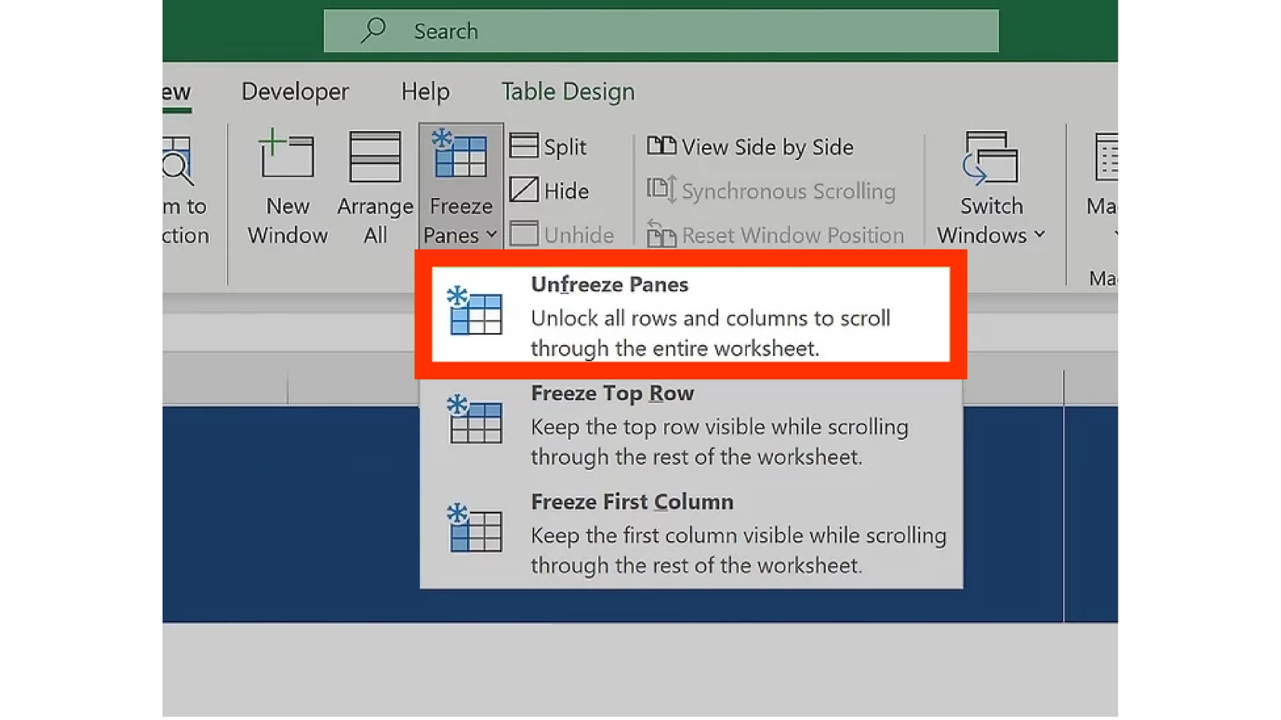
If you need to unfreeze the panes:
- Go to the View tab on the Ribbon.
- Click on Freeze Panes in the Window group.
- Select Unfreeze Panes from the dropdown menu.
This will remove all frozen panes in your spreadsheet.
Also read: A Comprehensive Guide on Advanced Microsoft Excel for Data Analysis
Practical Examples of Freezing Panes in Excel
Here are the examples:
Example 1: Freezing the Top Row for Data Entry
Let’s say you have a big dataset with headers (e.g., Name, Age, Department) on the first row, each representing a distinct item. By freezing the top row, you can ensure that the headers stay displayed while you enter data into the following rows.
Example 2: Freezing the First Column for Comparative Analysis
Let’s say you have a financial report that lists several financial metrics in the following columns and months in the first column. Comparing the first column is easier when it is frozen since you can scroll through the metrics and always see the month.
Example 3: Freezing Both Rows and Columns for Enhanced Readability
When you navigate a spreadsheet with both column headings and row labels—for example, a sales report with product names in the first column and sales regions in the top row freezing the first column and the top row makes it easier to maintain track of both dimensions of your data.
Tips for Using Freeze Panes Effectively
Here are tips for using freeze:
- Plan Your Layout: Determine which rows and columns are crucial for navigation and comparison before freezing panes.
- Use Split for More Flexibility: If you need even more freedom, you can use the Split tool (located under the View tab) to create separate scrollable sections.
- Incorporate with Additional Features: Combine Freeze Panes with other Excel capabilities, such as Filters, Tables, and Conditional Formatting, to improve your data analysis workflow.
Conclusion
Excel’s freezing panes are a straightforward but effective technique that improves your ability to explore and analyze big datasets. You can preserve context and increase productivity by making key rows and columns visible. Using Excel’s Freeze Panes tool will improve your productivity, whether you’re entering data, comparing metrics, or reading reports.
Frequently Asked Questions
Q1. Can I freeze panes on multiple sheets at once?
Ans. No, you need to freeze panes individually on each sheet where you want this feature enabled.
Q2. How do freezing panes affect printing?
Ans. Freezing panes does not affect how your worksheet is printed. If you want to repeat header rows or columns on each printed page, use the Page Layout tab and select Print Titles to set rows or columns to repeat.
Q3. Why do my frozen panes disappear when I switch to Page Layout view?
Ans. Frozen panes are not visible in the Page Layout view. To see them again, switch back to Normal view or Page Break Preview.
Q4. Do freezing panes affect formulas and data calculations?
Ans. Freezing panes does not affect formulas or data calculations. It only changes how you view the worksheet by keeping certain rows or columns visible while scrolling.
Q5. What are some best practices for using freeze panes?
Ans. Here are the best practices:
1. Identify Key Rows/Columns: Determine which rows or columns are most important for navigation and data comparison.
2. Combine with Other Features: For better data analysis, use freeze panes along with filters, tables, and conditional formatting.
3. Regular Updates: Regularly review and update frozen panes as your data and analysis needs change.
Hi, I am Janvi, a passionate data science enthusiast currently working at Analytics Vidhya. My journey into the world of data began with a deep curiosity about how we can extract meaningful insights from complex datasets.


