In this tutorial, you will learn how to construct iterate update and train a CNN model using JAX, Flax, and Optax on the MNIST dataset. This tutorial starts from how to set up the environment and preprocess the data to how to define the CNN structure and the final step is to test the model. It will also indicate how the core elements of JAX’s strong numerical performance, Flax’s flexible neural network, and Optax’s sophisticated optimization tools train and evaluate a state-of-the-art deep learning model efficiently. The goal of this guide is to explain how all these tools can be useful towards optimizing deep learning procedures and making models better.
Learning Objectives
- Learn how to integrate JAX, Flax, and Optax for efficient neural network construction.
- Understand the process of preprocessing and loading datasets using TensorFlow Datasets (TFDS).
- Implement a Convolutional Neural Network (CNN) for effective image classification.
- Visualize training progress with metrics like loss and accuracy.
- Evaluate and test the model on custom images for real-world applications.
This article was published as a part of the Data Science Blogathon.
Table of contents
- Learning Objectives
- JAX, Flax, and Optax: A Powerful Trio
- Getting Started with JAX: Installation and Setup
- Data Preparation: Loading and Preprocessing MNIST
- Building the Convolutional Neural Network (CNN)
- Model Evaluation: Metrics and Performance Tracking
- Implementing the Training Loop
- Executing the Training and Evaluation Process
- Visualizing Training and Testing Metrics
- Predicting Custom Images
- Conclusion
- Frequently Asked Questions
JAX, Flax, and Optax: A Powerful Trio
For deep learning models to be highly efficient and easily scalable, developers look for some valuable tools which help in computation, model designing and optimization. Guess what? Even with that assumption, there is still the question of how the three; JAX, Flax and Optax collectively address the challenges inherent in the development of complex ML models; well, let’s find out.
JAX: The Backbone of Numerical Computing
JAX is a high-performance numerical computing library with a familiar NumPy-like syntax. It excels in scenarios requiring hardware acceleration or automatic differentiation. Key features include:
- Autograd: Automatic differentiation for complex functions.
- JIT Compilation: Speeds up execution on CPUs, GPUs, or TPUs.
- Vectorization: Simplifies batch operations with tools like vmap.
- Hardware Integration: Optimized for GPUs and TPUs out of the box.
Flax: A Flexible Neural Network Library
Flax is a JAX-based library for building neural networks. It’s designed to be both user-friendly and customizable:
- Stateful Modules: Simplifies managing parameters and state.
- Compact API: Intuitive model definitions with the @nn.compact decorator.
- Customizability: Suitable for anything from simple to complex architectures.
- Seamless JAX Integration: Leverages JAX’s powerful features effortlessly.
Optax: A Comprehensive Optimization Library
Optax simplifies gradient processing and optimization, offering:
- Optimizers: A wide range, including SGD, Adam, and RMSProp.
- Gradient Processing: Tools for clipping, scaling, and normalization.
- Modularity: Easy composition of gradient transformations and optimizers.
Together, these libraries offer a powerful, modular ecosystem for building and training deep learning models efficiently.
Getting Started with JAX: Installation and Setup
However, to learn more about JAX and all of its capabilities, one must first start by implementing the structure on the system. Here, you will get a brief overview of how you can easily install JAX and get on with using these awesome features of JAX.
!pip install --upgrade -q pip jax jaxlib flax optax tensorflow-datasetsInstalls the required libraries:
- jax and jaxlib: Numerical computations on GPUs/TPUs.
- flax: Neural network library.
- optax: For optimization functions.
- tensorflow-datasets: Simplifies dataset loading.
Importing Essential Libraries for JAX, Flax, and Optax
To harness the power of JAX, Flax, and Optax, the first step is to import the necessary libraries into your development environment. This section will guide you through the process of importing these key libraries, ensuring that you have everything set up for the efficient execution of machine learning tasks. By correctly importing JAX, Flax, and Optax, you’re laying the foundation for creating high-performance models that can leverage advanced features like GPU/TPU acceleration and automatic differentiation. Let’s get started with the essential imports!
import jax
import jax.numpy as jnp               # JAX NumPy

from flax import linen as nn          # The Linen API
from flax.training import train_state
import optax                          # The Optax gradient processing and optimization library

import numpy as np                    # Ordinary NumPy
import tensorflow_datasets as tfds # TFDS for MNIST- JAX: For GPU-accelerated computations.
- Flax: To define and train the CNN.
- Optax: Provides optimizers like SGD.
- TFDS: Loads datasets like MNIST.
- Matplotlib: For visualizing training/testing metrics.
Data Preparation: Loading and Preprocessing MNIST
In this section, we will perform loading and preprocessing of the MNIST dataset which is being a standard dataset used in machine learning. MNIST dataset comprises of handwritten digits, by preparing this correctly, we ensure that the model is in a position to learn from the data. We will also describe how to import the dataset, resize the images and properly structure the data for training and assessment.
def get_datasets():
  ds_builder = tfds.builder('mnist')
  ds_builder.download_and_prepare()
  # Split into training/test sets
  train_ds = tfds.as_numpy(ds_builder.as_dataset(split='train', batch_size=-1))
  test_ds = tfds.as_numpy(ds_builder.as_dataset(split='test', batch_size=-1))
  # Convert to floating-points
  train_ds['image'] = jnp.float32(train_ds['image']) / 255.0
  test_ds['image'] = jnp.float32(test_ds['image']) / 255.0
  return train_ds, test_ds
train_ds, test_ds = get_datasets()We use TFDS to load and preprocess the MNIST dataset:
- The dataset includes 28×28 grayscale images of digits 0–9.
- Images are normalized by dividing pixel values by 255 to scale them between 0 and 1. This improves convergence during training.
The function returns train_ds and test_ds dictionaries with keys ‘image’ and ‘label’.

Building the Convolutional Neural Network (CNN)
CNNs is the architecture of choice for image classification problems, and in this section we will create a CNN in the jax + flax + optax stack. CNNs are expected to learn spatial hierarchies of image data by themselves due to layers of convolutions. This way, we will explain how to define layers, activation function’s layers, and the last layer which is the output layer for recognizing the digits in the MNIST data set.
class CNN(nn.Module):

  @nn.compact
  # Provide a constructor to register a new parameter
  # and return its initial value
  def __call__(self, x):
    x = nn.Conv(features=32, kernel_size=(3, 3))(x)
    x = nn.relu(x)
    x = nn.avg_pool(x, window_shape=(2, 2), strides=(2, 2))
    x = nn.Conv(features=64, kernel_size=(3, 3))(x)
    x = nn.relu(x)
    x = nn.avg_pool(x, window_shape=(2, 2), strides=(2, 2))
    x = x.reshape((x.shape[0], -1)) # Flatten
    x = nn.Dense(features=256)(x)
    x = nn.relu(x)
    x = nn.Dense(features=10)(x)    # There are 10 classes in MNIST
return x- Convolution Layers: Extract features using nn.Conv. And add non-linearity using nn.relu.
- Pooling Layers: Perform dimensionality reduction using nn.avg_pool.
- Flatten Layer: Convert feature maps into a 1D vector.
- Dense Layers: A fully connected layer with 256 neurons for feature learning. An output layer with 10 neurons for MNIST classification.
Model Evaluation: Metrics and Performance Tracking
After our Convolutional Neural Network (CNN) has been trained properly, we need to evaluate its performance and do so using the right measures. Now we will discuss about the major observations regarding the model accuracy, loss, etc., specifically on the training and validation set.
def compute_metrics(logits, labels):
  loss = jnp.mean(optax.softmax_cross_entropy(logits, jax.nn.one_hot(labels, num_classes=10)))
  accuracy = jnp.mean(jnp.argmax(logits, -1) == labels)
  metrics = {
      'loss': loss,
      'accuracy': accuracy
  }
  return metrics
We define metrics to evaluate model performance:
- Loss: Calculated using optax.softmax_cross_entropy. It measures the difference between predicted and actual labels.
- Accuracy: Measures the fraction of correctly predicted labels using jnp.argmax.
The function returns train_ds and test_ds dictionaries with keys ‘image’ and ‘label’.
Training and Evaluation Functions
We define the functions responsible for training the model on the dataset and evaluating its performance. These functions handle the forward pass, loss calculation, backpropagation, and tracking the model’s accuracy during both training and validation phases.
@jax.jit
def train_step(state, batch):
  def loss_fn(params):
    logits = CNN().apply({'params': params}, batch['image'])
    loss = jnp.mean(optax.softmax_cross_entropy(
        logits=logits,
        labels=jax.nn.one_hot(batch['label'], num_classes=10)))
    return loss, logits
  grad_fn = jax.value_and_grad(loss_fn, has_aux=True)
  (_, logits), grads = grad_fn(state.params)
  state = state.apply_gradients(grads=grads)
  metrics = compute_metrics(logits, batch['label'])
  return state, metrics

@jax.jit
def eval_step(params, batch):
  logits = CNN().apply({'params': params}, batch['image'])
  return compute_metrics(logits, batch['label'])
Training Step:
- Computes the loss and gradients with respect to model parameters using jax.value_and_grad().
- Updates the model parameters using the optimizer.
- Returns the updated state and metrics for tracking performance.
Evaluation Step:
- Evaluates the model using the given batch.
- Computes the metrics (loss and accuracy) using the trained parameters.
Both functions are JIT-compiled for faster performance execution.
Implementing the Training Loop
We integrate the training process into a loop that iteratively trains the model over multiple epochs. During each iteration, the model is updated based on the computed gradients, and performance metrics are tracked to ensure steady progress towards optimization.
def train_epoch(state, train_ds, batch_size, epoch, rng):
  train_ds_size = len(train_ds['image'])
  steps_per_epoch = train_ds_size // batch_size

  perms = jax.random.permutation(rng, len(train_ds['image']))
  perms = perms[:steps_per_epoch * batch_size]  # Skip an incomplete batch
  perms = perms.reshape((steps_per_epoch, batch_size))

  batch_metrics = []

  for perm in perms:
    batch = {k: v[perm, ...] for k, v in train_ds.items()}
    state, metrics = train_step(state, batch)
    batch_metrics.append(metrics)

  training_batch_metrics = jax.device_get(batch_metrics)
  training_epoch_metrics = {
      k: np.mean([metrics[k] for metrics in training_batch_metrics])
      for k in training_batch_metrics[0]}

  print('Training - epoch: %d, loss: %.4f, accuracy: %.2f' % (epoch, training_epoch_metrics['loss'], training_epoch_metrics['accuracy'] * 100))

return state, training_epoch_metrics- Computes the number of training steps based on the batch size.
- Shuffles the dataset and prepares batches using jax.random.permutation.
- For each batch, train_step is called to update the model.
- At the end of each epoch, it calculates and logs the average training loss and accuracy.
Evaluate the Model
def eval_model(model, test_ds):
  metrics = eval_step(model, test_ds)
  metrics = jax.device_get(metrics)
  eval_summary = jax.tree.map(lambda x: x.item(), metrics)
return eval_summary['loss'], eval_summary['accuracy']- Computes the loss and accuracy on the test data using eval_step.
- Returns the evaluation result(loss and accuracy).
Executing the Training and Evaluation Process
This step involves running the training loop and during each epoch the model performance has to be tested. By checking the training and validation metrics, we make sure that the model learning process is going on and, moreover, the model’s ability to generalize data that it has never encountered before.
rng = jax.random.PRNGKey(0)
rng, init_rng = jax.random.split(rng)

cnn = CNN()
params = cnn.init(init_rng, jnp.ones([1, 28, 28, 1]))['params']

nesterov_momentum = 0.9
learning_rate = 0.001
tx = optax.sgd(learning_rate=learning_rate, nesterov=nesterov_momentum)

state = train_state.TrainState.create(apply_fn=cnn.apply, params=params, tx=tx)

# Initialize lists to store metrics for graph visualization
training_losses = []
training_accuracies = []
testing_losses = []
testing_accuracies = []
num_epochs = 10
batch_size = 64

for epoch in range(1, num_epochs + 1):
  # Use a separate PRNG key to permute image data during shuffling
  rng, input_rng = jax.random.split(rng)
  # Run an optimization step over a training batch
  state, train_metrics = train_epoch(state, train_ds, batch_size, epoch, input_rng)
  # Evaluate on the test set after each training epoch
  test_loss, test_accuracy = eval_model(state.params, test_ds)
  print('Testing - epoch: %d, loss: %.2f, accuracy: %.2f' % (epoch, test_loss, test_accuracy * 100))
  # Store metrics for graph visualization
  training_losses.append(train_metrics['loss'])
  training_accuracies.append(train_metrics['accuracy'])
  testing_losses.append(test_loss)
  testing_accuracies.append(test_accuracy)
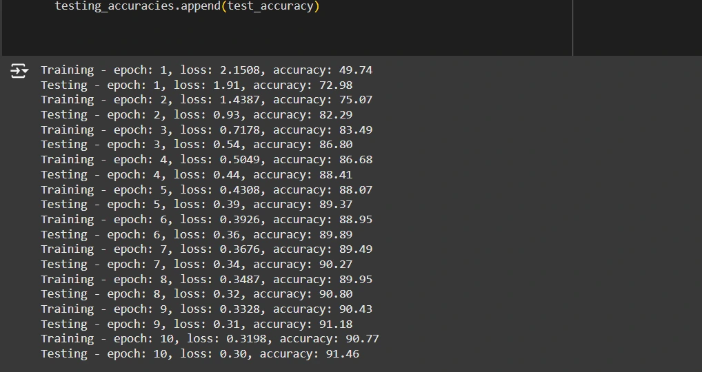
- RNG Initialization: Set up a random number generator (rng) for reproducibility and randomness in data shuffling and parameter initialization.
- Model Initialization: Create the CNN model and initialize its parameters using a dummy input.
- Optimizer and Training State:
- Use optax.sgd as the optimizer with a learning rate of 0.001 and Nesterov momentum of 0.9.
- Store the model parameters and optimizer in the TrainState.
- Training Loop:
- Shuffle the training data using a new random key (input_rng).
- Train the model using train_epoch for one full pass through the dataset.
- Evaluate the model on the test dataset using eval_step.
- Print Metrics: Log the test loss and accuracy after each epoch.
Visualizing Training and Testing Metrics
In this step, we visualize the training and testing metrics such as accuracy and loss over time. This helps to identify trends, diagnose potential issues like overfitting or underfitting, and assess the overall performance of the model during training.
import matplotlib.pyplot as plt
# Graph visualization for training/testing loss and accuracy
epochs = range(1, num_epochs + 1)

plt.figure(figsize=(14, 5))

# Plot for Loss
plt.subplot(1, 2, 1)
plt.plot(epochs, training_losses, label='Training Loss', marker='o')
plt.plot(epochs, testing_losses, label='Testing Loss', marker='o')
plt.title('Loss Over Epochs')
plt.xlabel('Epochs')
plt.ylabel('Loss')
plt.legend()
plt.grid(True)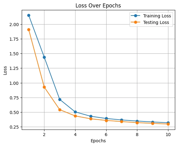
Predicting Custom Images
We will now demonstrate how to use the trained model to make predictions on custom images. This allows you to evaluate the model’s performance on unseen data and test its ability to generalize to new, real-world examples.
from google.colab import files
from PIL import Image
import numpy as np

# Step 1: Upload the image file
uploaded = files.upload()

# Step 2: Process the uploaded image
def load_and_preprocess_image(file_path):
    img = Image.open(file_path).convert('L')  # Convert to grayscale
    img = img.resize((28, 28))               # Resize to 28x28
    img = np.array(img) / 255.0              # Normalize pixel values to [0, 1]
    img = img.reshape(1, 28, 28, 1)          # Add batch and channel dimensions
    return img

# Step 3: Load and preprocess each uploaded image
for file_name in uploaded.keys():
    test_image = load_and_preprocess_image(file_name)
    print(f"Processed image from {file_name}.")


import jax.numpy as jnp

# Convert to JAX array
test_image_jax = jnp.array(test_image, dtype=jnp.float32)

# Step 4: Use your trained model for predictions
logits = state.apply_fn({'params': state.params}, test_image_jax)
prediction = jnp.argmax(logits, axis=-1)
print(f"Predicted class: {prediction[0]}")


# Display the uploaded image
plt.imshow(test_image[0].squeeze(), cmap='gray')
plt.title(f"Predicted Class: {prediction[0]}")
plt.axis('off')
plt.show()
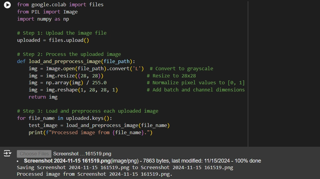
Uploading Images
- The first step is to upload the custom handwritten digit images.
- The files.upload() function opens a file upload interface in the Colab environment to enable uploading.
- It allows users to select one or more images from their local machine in a supported format (e.g., PNG, JPG).
- Once uploaded, the files are accessible for further processing in the code.
Preprocessing
After uploading, the model processes the images to match the expected input format.
- Convert to Grayscale: We convert the image to grayscale using `Image.convert(‘L’)`, as MNIST images are single-channel.
- Resize to 28×28 Pixels: The image is resized to the standard MNIST dimensions using Image.resize((28, 28)).
- Normalize Pixel Values: We scale the pixel values to the range [0, 1] by dividing by 255.0 to ensure consistent input values.
- Reshape for Model Input: We reshape the image into a tensor with dimensions [1, 28, 28, 1] to include the batch size and channel dimensions.
Prediction
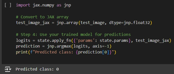
- We convert the preprocessed image into a JAX-compatible array (jnp.array), optimizing it for efficient computation.
- We pass this array through the trained model using the apply_fn function, which computes the logits (raw output scores for each class).
- We use jnp.argmax to find the index of the maximum logit value, which corresponds to the class with the highest confidence.
Visualization
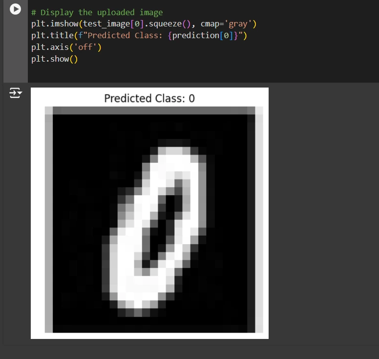
- The processed image is displayed using Matplotlib to provide a visual reference for the user.
- The predicted class is displayed as the image’s title for easy interpretation of the results.
- This visualization step helps validate the model’s predictions and makes the classification process intuitive and user-friendly.
Conclusion
This step-by-step guide demonstrated the power and flexibility of JAX, Flax, and Optax in building a robust deep learning pipeline for image classification. By leveraging their unique features like efficient hardware acceleration, modular design, and advanced optimization capabilities, we trained a Convolutional Neural Network (CNN) on the dataset with ease. The integration with TensorFlow Datasets (TFDS) simplified data loading and preprocessing, while visualizing metrics provided valuable insights into the model’s performance.
The pipeline culminated in testing the model on custom images, showcasing its practical application. This approach is not only scalable for more complex datasets but also serves as a foundation for exploring cutting-edge deep learning techniques.
Here is the collab link: Click Here.
Key Takeaways
- JAX, Flax, and Optax provide powerful tools for efficient deep learning model building and optimization.
- Data preprocessing and augmentation are essential for enhancing model performance on real-world datasets.
- Convolutional Neural Networks (CNNs) are effective for image classification tasks like MNIST.
- Evaluating model performance with appropriate metrics helps track improvements and identify areas for refinement.
- Visualizing training and testing metrics provides valuable insights into model behavior and progress during training.
Frequently Asked Questions
A. JAX is a high-performance numerical computing library that offers features like automatic differentiation and GPU/TPU acceleration. We use it here to efficiently compute gradients and execute deep learning operations seamlessly on hardware accelerators.
A. Flax is a lightweight, modular library built on JAX, designed for flexibility and scalability. Its @compact API simplifies model definitions, making it easier to experiment with different architectures while leveraging JAX’s powerful features.
A. Optax offers a comprehensive suite of optimization algorithms and tools for gradient processing, such as SGD with momentum, which efficiently trains the CNN.
A. TFDS simplifies dataset handling by providing pre-built datasets like MNIST, along with tools for automatic downloading, preprocessing, and splitting into training and testing sets.
The media shown in this article is not owned by Analytics Vidhya and is used at the Author’s discretion.


