Comparing a CART model to Random Forest (Part 1)

I created my first simple regression model with my father in 8th standard (year: 2002) on MS Excel. Obviously, my contribution in that model was minimal, but I really enjoyed the graphical representation of the data. We tried validating all the assumptions etc. for this model. By the end of the exercise, we had 5 sheets of the simple regression model on 700 data points. The entire exercise was complex enough to confuse any person with average IQ level. When I look at my models today, which are built on millions of observations and utilize complex statistics behind the scene, I realize how machine learning with sophisticated tools (like SAS, SPSS, R)  has made our life easy.

Having said that, many people in the industry do not bother about the complex statistics, which goes behind the scene. It becomes very important to realize the predictive power of each technique. No model is perfect in all scenarios. Hence, we need to understand the data and the surrounding eco-system before coming up with a model recommendation.

In this article, we will compare two widely used techniques i.e. CART vs. Random forest. Basics of Random forest were covered in my last article. We will take a case study to build a strong foundation of this concept and use R to do the comparison. The dataset used in this article is an inbuilt dataset of R.

As the concept is pretty lengthy, we have broken down this article into two parts

[stextbox id=”section”] Background on Dataset “Iris” [/stextbox]

Data set “iris” gives the measurements in centimeters of the variables : sepal length and width and petal length and width, respectively, for 50 flowers from each of 3 species of Iris. The dataset has 150 cases (rows) and 5 variables (columns) named Sepal.Length, Sepal.Width, Petal.Length, Petal.Width, Species. We intend to predict the Specie based on the 4 flower characteristic variables.

We will first load the dataset into R and then look at some of the key statistics. You can use the following codes to do so.

data(iris)

# look at the dataset

summary(iris)

# visually look at the dataset

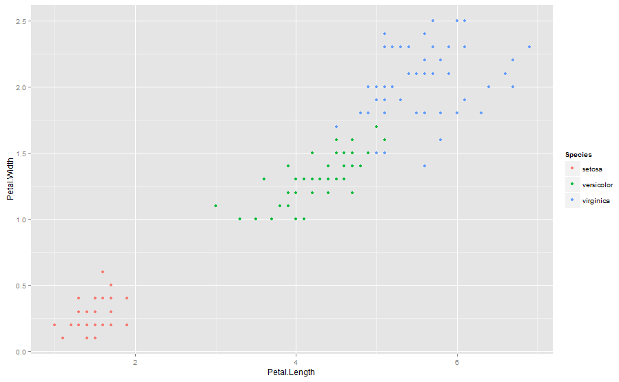
qplot(Petal.Length,Petal.Width,colour=Species,data=iris)

The three species seem to be well segregated from each other. The accuracy in prediction of borderline cases determines the predictive power of the model. In this case, we will install two useful packages for making a CART model.

library(rpart)

library(caret)

After loading the library, we will divide the population in two sets: Training and validation. We do this to make sure that we do not overfit the model. In this case, we use a split of 50-50 for training and validation. Generally, we keep training heavier to make sure that we capture the key characteristics. You can use the following code to make this split.

train.flag <- createDataPartition(y=iris$Species,p=0.5,list=FALSE)

training <- iris[train.flag,]

Validation <- iris[-train.flag,]

[stextbox id=”section”] Building a CART model [/stextbox]

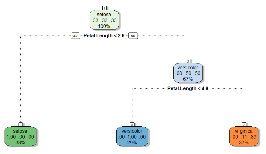
Once we have the two data sets and have got a basic understanding of data, we now build a CART model. We have used “caret” and “rpart” package to build this model. However, the traditional representation of the CART model is not graphically appealing on R. Hence, we have used a package called “rattle” to make this decision tree. “Rattle” builds a more fancy and clean trees, which can be easily interpreted. Use the following code to build a tree and graphically check this tree:

modfit <- train(Species~.,method="rpart",data=training) 

library(rattle)

fancyRpartPlot(modfit$finalModel)

[stextbox id=”section”] Validating the model [/stextbox]

Now, we need to check the predictive power of the CART model, we just built. Here, we are looking at a discordance rate (which is the number of misclassifications in the tree) as the decision criteria. We use the following code to do the same :

train.cart<-predict(modfit,newdata=training)

table(train.cart,training$Species)

train.cart   setosa versicolor virginica

setosa         25         0         0

versicolor     0         22         0

virginica       0         3       25

# Misclassification rate = 3/75

Only 3 misclassified observations out of 75, signifies good predictive power. In general, a model with misclassification rate less than 30% is considered to be a good model. But, the range of a good model depends on the industry and the nature of the problem. Once we have built the model, we will validate the same on a separate data set. This is done to make sure that we are not over fitting the model. In case we do over fit the model, validation will show a sharp decline in the predictive power. It is also recommended to do an out of time validation of the model. This will make sure that our model is not time dependent. For instance, a model built in festive time, might not hold in regular time. For simplicity, we will only do an in-time validation of the model. We use the following code to do an in-time validation:

pred.cart<-predict(modfit,newdata=Validation)

table(pred.cart,Validation$Species)

pred.cart   setosa versicolor virginica

setosa         25         0         0

versicolor     0         22         1

virginica       0         3       24

# Misclassification rate = 4/75

As we see from the above calculations that the predictive power decreased in validation as compared to training. This is generally true in most cases. The reason being, the model is trained on the training data set, and just overlaid on validation training set. But, it hardly matters, if the predictive power of validation is lesser or better than training. What we need to check is that they are close enough. In this case, we do see the misclassification rate to be really close to each other. Hence, we see a stable CART model in this case study.

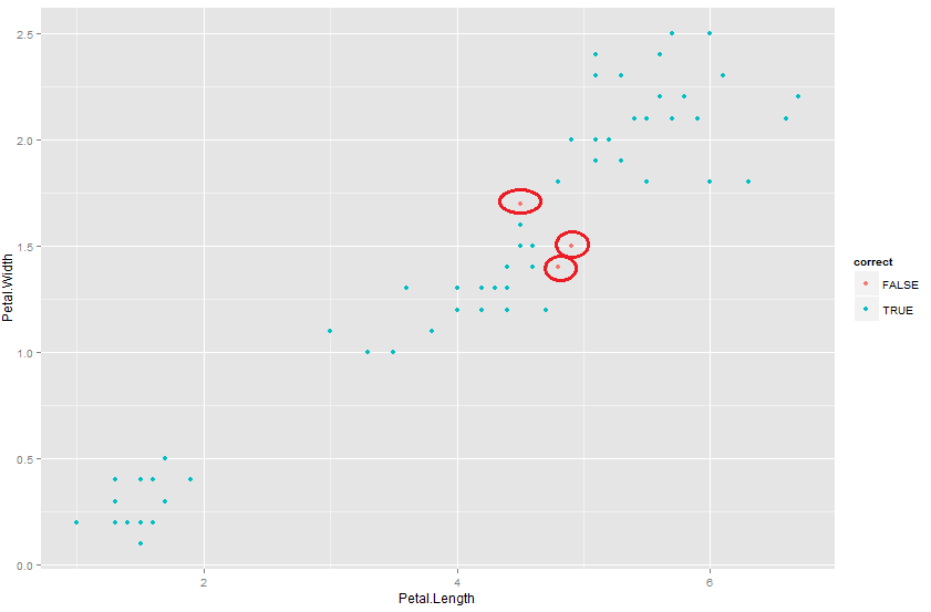
Let’s now try to visualize the cases for which the prediction went wrong. Following is the code we use to find the same :

correct <- pred.cart == Validation$Species

qplot(Petal.Length,Petal.Width,colour=correct,data=Validation)

As you see from the graph, the predictions which went wrong were actually those borderline cases. We have already discussed before that these are the cases which make or break the comparison for the model. Most of the models will be able to categorize observation far away from each other. It takes a model to be sharp to distinguish these borderline cases.

[stextbox id=”section”]End Notes : [/stextbox]

In the next article, we will solve the same problem using a random forest algorithm. We hope that random forest will be able to make even better prediction for these borderline cases. But, we can never generalize the order of predictive power among a CART and a random forest, or rather any predictive algorithm. The reason being every model has its own strength. Random forest generally tends to have a very high accuracy on the training population, because it uses many different characteristics to make a prediction. But, because of the same reason, it sometimes over fits the model on the data. We will see these observations graphically in the next article and talk in more details on scenarios where random forest or CART comes out to be a better predictive model.

Did you find the article useful? Did this article solve any of your existing dilemmas? Have you compared the two models in any of your projects? If you did, share with us your thoughts on the topic.

If you like what you just read & want to continue your analytics learning, subscribe to our emails, follow us on twitter or like our facebook page.

Tavish Srivastava

Tavish Srivastava, co-founder and Chief Strategy Officer of Analytics Vidhya, is an IIT Madras graduate and a passionate data-science professional with 8+ years of diverse experience in markets including the US, India and Singapore, domains including Digital Acquisitions, Customer Servicing and Customer Management, and industry including Retail Banking, Credit Cards and Insurance. He is fascinated by the idea of artificial intelligence inspired by human intelligence and enjoys every discussion, theory or even movie related to this idea.