Learn how to Build your own Speech-to-Text Model (using Python)

Overview

• Learn how to build your very own speech-to-text model using Python in this article
• The ability to weave deep learning skills with NLP is a coveted one in the industry; add this to your skillset today
• We will use a real-world dataset and build this speech-to-text model so get ready to use your Python skills!

Introduction

“Hey Google. What’s the weather like today?”

This will sound familiar to anyone who has owned a smartphone in the last decade. I can’t remember the last time I took the time to type out the entire query on Google Search. I simply ask the question – and Google lays out the entire weather pattern for me.

It saves me a ton of time and I can quickly glance at my screen and get back to work. A win-win for everyone! But how does Google understand what I’m saying? And how does Google’s system convert my query into text on my phone’s screen?

This is where the beauty of speech-to-text models comes in. Google uses a mix of deep learning and Natural Language Processing (NLP) techniques to parse through our query, retrieve the answer and present it in the form of both audio and text.

The same speech-to-text concept is used in all the other popular speech recognition technologies out there, such as Amazon’s Alexa, Apple’s Siri, and so on. The semantics might vary from company to company, but the overall idea remains the same.

I have personally researched quite a bit on this topic as I wanted to understand how I could build my own speech-to-text model using my Python and deep learning skills. It’s a fascinating concept and one I wanted to share with all of you.

So in this article, I will walk you through the basics of speech recognition systems (AKA an introduction to signal processing). We will then use this as the core when we implement our own speech-to-text model from scratch in Python.

Looking for a place to start your deep learning and/or NLP journey? We’ve got the perfect resources for you:

• Computer Vision using Deep Learning 2.0 Course
• Natural Language Processing (NLP) using Python

A Brief History of Speech Recognition through the Decades

You must be quite familiar with speech recognition systems. They are ubiquitous these days – from Apple’s Siri to Google Assistant. These are all new advents though brought about by rapid advancements in technology.

Did you know that the exploration of speech recognition goes way back to the 1950s? That’s right – these systems have been around for over 50 years! We have prepared a neat illustrated timeline for you to quickly understand how Speech Recognition systems have evolved over the decades:

• The first speech recognition system, Audrey, was developed back in 1952 by three Bell Labs researchers. Audrey was designed to recognize only digits
• Just after 10 years, IBM introduced its first speech recognition system IBM Shoebox, which was capable of recognizing 16 words including digits. It could identify commands like  “Five plus three plus eight plus six plus four minus nine, total,” and would print out the correct answer, i.e., 17
• The Defense Advanced Research Projects Agency (DARPA) contributed a lot to speech recognition technology during the 1970s. DARPA funded for around 5 years from 1971-76 to a program called Speech Understanding Research and finally, Harpy was developed which was able to recognize 1011 words. It was quite a big achievement at that time.
• In the 1980s, the Hidden Markov Model (HMM) was applied to the speech recognition system. HMM is a statistical model which is used to model the problems that involve sequential information. It has a pretty good track record in many real-world applications including speech recognition. 
• In 2001, Google introduced the Voice Search application that allowed users to search for queries by speaking to the machine.  This was the first voice-enabled application which was very popular among the people. It made the conversation between the people and machines a lot easier. 
• By 2011, Apple launched Siri that offered a real-time, faster, and easier way to interact with the Apple devices by just using your voice. As of now, Amazon’s Alexa and Google’s Home are the most popular voice command based virtual assistants that are being widely used by consumers across the globe. 

Wouldn’t it be great if we can also work on such great use cases using our machine learning skills? That’s exactly what we will be doing in this tutorial!

Introduction to Signal Processing

Before we dive into the practical aspect of speech-to-text systems, I strongly recommend reading up on the basics of signal processing first. This will enable you to understand how the Python code works and make you a better NLP and deep learning professional!

So, let us first understand some common terms and parameters of a signal.

What is an Audio Signal?

This is pretty intuitive – any object that vibrates produces sound waves. Have you ever thought of how we are able to hear someone’s voice? It is due to the audio waves. Let’s quickly understand the process behind it.

When an object vibrates, the air molecules oscillate to and fro from their rest position and transmits its energy to neighboring molecules. This results in the transmission of energy from one molecule to another which in turn produces a sound wave.

Parameters of an audio signal

• Amplitude: Amplitude refers to the maximum displacement of the air molecules from the rest position
• Crest and Trough: The crest is the highest point in the wave whereas trough is the lowest point
• Wavelength: The distance between 2 successive crests or troughs is known as a wavelength

• Cycle: Every audio signal traverses in the form of cycles. One complete upward movement and downward movement of the signal form a cycle
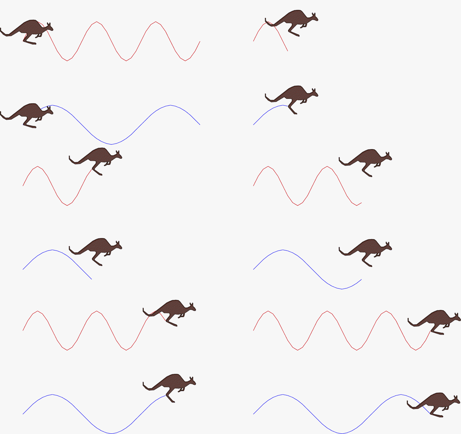
• Frequency: Frequency refers to how fast a signal is changing over a period of time

The below GIF wonderfully depicts the difference between a high and low-frequency signal:

In the next section, I will discuss different types of signals that we encounter in our daily life.

Different types of signals

We come across broadly two different types of signals in our day-to-day life – Digital and Analog.

Digital signal

A digital signal is a discrete representation of a signal over a period of time. Here, the finite number of samples exists between any two-time intervals.

For example, the batting average of top and middle-order batsmen year-wise forms a digital signal since it results in a finite number of samples.

Analog signal

An analog signal is a continuous representation of a signal over a period of time. In an analog signal, an infinite number of samples exist between any two-time intervals.

For example, an audio signal is an analog one since it is a continuous representation of the signal.

Wondering how we are going to store the audio signal since it has an infinite number of samples? Sit back and relax! We will touch on that concept in the next section.

What is sampling the signal and why is it required?

An audio signal is a continuous representation of amplitude as it varies with time. Here, time can even be in picoseconds. That is why an audio signal is an analog signal.

Analog signals are memory hogging since they have an infinite number of samples and processing them is highly computationally demanding. Therefore, we need a technique to convert analog signals to digital signals so that we can work with them easily.

Sampling the signal is a process of converting an analog signal to a digital signal by selecting a certain number of samples per second from the analog signal. Can you see what we are doing here? We are converting an audio signal to a discrete signal through sampling so that it can be stored and processed efficiently in memory.

I really like the below illustration. It depicts how the analog audio signal is discretized and stored in the memory:

The key thing to take away from the above figure is that we are able to reconstruct an almost similar audio wave even after sampling the analog signal since I have chosen a high sampling rate. The sampling rate or sampling frequency is defined as the number of samples selected per second. 

Different Feature Extraction Techniques for an Audio Signal

The first step in speech recognition is to extract the features from an audio signal which we will input to our model later. So now, l will walk you through the different ways of extracting features from the audio signal.

Time-domain

Here, the audio signal is represented by the amplitude as a function of time. In simple words, it is a plot between amplitude and time. The features are the amplitudes which are recorded at different time intervals.

The limitation of the time-domain analysis is that it completely ignores the information about the rate of the signal which is addressed by the frequency domain analysis. So let’s discuss that in the next section.

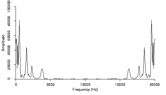
Frequency domain

In the frequency domain, the audio signal is represented by amplitude as a function of frequency. Simply put – it is a plot between frequency and amplitude. The features are the amplitudes recorded at different frequencies.

The limitation of this frequency domain analysis is that it completely ignores the order or sequence of the signal which is addressed by time-domain analysis.

Remember:

Time-domain analysis completely ignores the frequency component whereas frequency domain analysis pays no attention to the time component.

We can get the time-dependent frequencies with the help of a spectrogram.

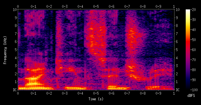
Spectrogram

Ever heard of a spectrogram? It’s a 2D plot between time and frequency where each point in the plot represents the amplitude of a particular frequency at a particular time in terms of intensity of color. In simple terms, the spectrogram is a spectrum (broad range of colors) of frequencies as it varies with time. 

The right features to extract from audio depends on the use case we are working with. It’s finally time to get our hands dirty and fire up our Jupyter Notebook!

Understanding the Problem Statement for our Speech-to-Text Project

Let’s understand the problem statement of our project before we move into the implementation part.

We might be on the verge of having too many screens around us. It seems like every day, new versions of common objects are “re-invented” with built-in wifi and bright touchscreens. A promising antidote to our screen addiction is voice interfaces. 

TensorFlow recently released the Speech Commands Datasets. It includes 65,000 one-second long utterances of 30 short words, by thousands of different people. We’ll build a speech recognition system that understands simple spoken commands.

You can download the dataset from here.

Implementing the Speech-to-Text Model in Python

The wait is over! It’s time to build our own Speech-to-Text model from scratch.

Import the libraries

First, import all the necessary libraries into our notebook. LibROSA and SciPy are the Python libraries used for processing audio signals.

Python Code:

import os
import librosa   #for audio processing
import IPython.display as ipd
import matplotlib.pyplot as plt
import numpy as np
from scipy.io import wavfile #for audio processing
import warnings
warnings.filterwarnings("ignore")

Visualization of Audio signal in time series domain

Now, we’ll visualize the audio signal in the time series domain:

Sampling rate

Let us now look at the sampling rate of the audio signals:

ipd.Audio(samples, rate=sample_rate)
print(sample_rate)

Resampling

From the above, we can understand that the sampling rate of the signal is 16,000 Hz. Let us re-sample it to 8000 Hz since most of the speech-related frequencies are present at 8000 Hz:

samples = librosa.resample(samples, sample_rate, 8000)
ipd.Audio(samples, rate=8000)

Now, let’s understand the number of recordings for each voice command:

Duration of recordings

What’s next? A look at the distribution of the duration of recordings:

Preprocessing the audio waves

In the data exploration part earlier, we have seen that the duration of a few recordings is less than 1 second and the sampling rate is too high. So, let us read the audio waves and use the below-preprocessing steps to deal with this.

Here are the two steps we’ll follow:

• Resampling
• Removing shorter commands of less than 1 second

Let us define these preprocessing steps in the below code snippet:

Convert the output labels to integer encoded:

Now, convert the integer encoded labels to a one-hot vector since it is a multi-classification problem:

from keras.utils import np_utils
y=np_utils.to_categorical(y, num_classes=len(labels))

Reshape the 2D array to 3D since the input to the conv1d must be a 3D array:

all_wave = np.array(all_wave).reshape(-1,8000,1)

Split into train and validation set

Next, we will train the model on 80% of the data and validate on the remaining 20%:

from sklearn.model_selection import train_test_split
x_tr, x_val, y_tr, y_val = train_test_split(np.array(all_wave),np.array(y),stratify=y,test_size = 0.2,random_state=777,shuffle=True)

Model Architecture for this problem

We will build the speech-to-text model using conv1d. Conv1d is a convolutional neural network which performs the convolution along only one dimension. 

Here is the model architecture:

Model building

Let us implement the model using Keras functional API.

Define the loss function to be categorical cross-entropy since it is a multi-classification problem:

model.compile(loss='categorical_crossentropy',optimizer='adam',metrics=['accuracy'])

Early stopping and model checkpoints are the callbacks to stop training the neural network at the right time and to save the best model after every epoch:

es = EarlyStopping(monitor='val_loss', mode='min', verbose=1, patience=10, min_delta=0.0001) 
mc = ModelCheckpoint('best_model.hdf5', monitor='val_acc', verbose=1, save_best_only=True, mode='max')

Let us train the model on a batch size of 32 and evaluate the performance on the holdout set:

history=model.fit(x_tr, y_tr ,epochs=100, callbacks=[es,mc], batch_size=32, validation_data=(x_val,y_val))

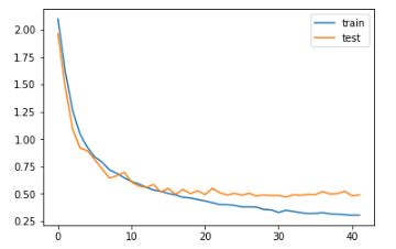
Diagnostic plot

I’m going to lean on visualization again to understand the performance of the model over a period of time:

Loading the best model

from keras.models import load_model
model=load_model('best_model.hdf5')

Define the function that predicts text for the given audio:

Prediction time! Make predictions on the validation data:

The best part is yet to come! Here is a script that prompts a user to record voice commands. Record your own voice commands and test it on the model:

Let us now read the saved voice command and convert it to text:

Here is an awesome video that I tested on one of my colleague’s voice commands:

Congratulations! You have just built your very own speech-to-text model!

Frequently Asked Questions

Code

Find the notebook here

End Notes

Got to love the power of deep learning and NLP. This is a microcosm of the things we can do with deep learning. I encourage you to try it out and share the results with our community. 🙂

In this article, we covered all the concepts and implemented our own speech recognition system from scratch in Python.

I hope you have learned something new today. I will see you in the next article. If you have any queries/feedback, please free to share in the below comments section!

Aravind Pai

Aravind Pai is passionate about building data-driven products for the sports domain. He strongly believes that Sports Analytics is a Game Changer.