Introduction
One of the most basic concepts in statistics is hypothesis testing. Not just in Data Science, Hypothesis testing is important in every field. Want to know how??? Let us take an example. You must have heard about lifebuoy?? Suppose
lifebuoy claims that, it kills 99.9% of germs. So how can they say so? There has to be a testing technique to prove this claim right?? So hypothesis testing uses to prove a claim or any assumptions.
Table of Content
- Definition of Hypothesis Testing.
- Null and Alternative Hypothesis Testing
- Simple and composite Hypothesis Testing
- One-tailed and two-tailed testing
- Critical Region.
- Type I and Type II error.
- Statistically significant.
- Level of confidence
- Level of significance
- P-value.
This blog breaks these concepts down into small pieces so that you can understand their motivation and their uses. By the time you’re done with this blog, Hypothesis Testing basics will be clear!!!
Definition of Hypothesis Testing
The hypothesis is a statement, assumption or claim about the value of the parameter (mean, variance, median etc.).
A hypothesis is an educated guess about something in the world around you. It should be testable, either by experiment or observation.
Like, if we make a statement that “Dhoni is the best Indian Captain ever.” This is an assumption that we are making based on the average wins and losses team had under his captaincy. We can test this statement based on all the match data.
Null and Alternative Hypothesis Testing
The null hypothesis is the hypothesis to be tested for possible rejection under the assumption that it is true. The concept of the null is similar to innocent until proven guilty We assume innocence until we have enough evidence to prove that a suspect is guilty.
In simple language, we can understand the null hypothesis as already accepted statements, For example, Sky is blue. We already accept this statement.
It is denoted by H0.
The alternative hypothesis complements the Null hypothesis. It is the opposite of the null hypothesis such that both Alternate and null hypothesis together cover all the possible values of the population parameter.
It is denoted by H1.
Let’s understand this with an example:
A soap company claims that its product kills on an average of 99% of the germs. To test the claim of this company we will formulate the null and alternate hypothesis.
Null Hypothesis(H0): Average =99%
Alternate Hypothesis(H1): Average is not equal to 99%.
Note: When we test a hypothesis, we assume the null hypothesis to be true until there is sufficient evidence in the sample to prove it false. In that case, we reject the null hypothesis and support the alternate hypothesis. If the sample fails to provide sufficient evidence for us to reject the null hypothesis, we cannot say that the null hypothesis is true because it is based on just the sample data. For saying the null hypothesis is true we will have to study the whole population data.
Simple and Composite Hypothesis Testing
When a hypothesis specifies an exact value of the parameter, it is a simple hypothesis and if it specifies a range of values then it is called a composite hypothesis.
e.g. Motor cycle company claiming that a certain model gives an average mileage of 100Km per liter, this is a case of simple hypothesis.
The average age of students in a class is greater than 20. This statement is a composite hypothesis.
One-tailed and two-tailed Hypothesis Testing
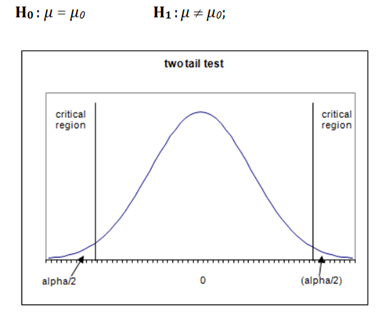
If the alternate hypothesis gives the alternate in both directions (less than and greater than) of the value of the parameter specified in the null hypothesis, it is called a Two-tailed test.
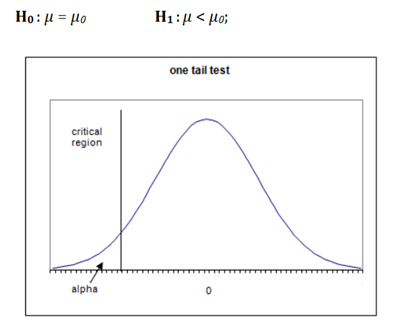
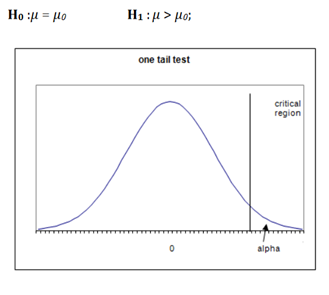
If the alternate hypothesis gives the alternate in only one direction (either less than or greater than) of the value of the parameter specified in the null hypothesis, it is called a One-tailed test.
e.g. if H0: mean= 100 H1: mean not equal to 100
here according to H1, mean can be greater than or less than 100. This is an example of a Two-tailed test
Similarly, if H0: mean>=100 then H1: mean< 100
Here, the mean is less than 100. It is called a One-tailed test.
Critical Region
The critical region is that region in the sample space in which if the calculated value lies then we reject the null hypothesis.
Let’s understand this with an example:
Suppose you are looking to rent an apartment. You listed out all the available apartments from different real state websites. You have a budget of Rs. 15000/ month. You cannot spend more than that. The list of apartments you have made has a price ranging from 7000/month to 30,000/month.
You select a random apartment from the list and assume below hypothesis:
H0: You will rent the apartment.
H1: You won’t rent the apartment.
Now, since your budget is 15000, you have to reject all the apartments above that price.
Here all the Prices greater than 15000 become your critical region. If the random apartment’s price lies in this region, you have to reject your null hypothesis and if the random apartment’s price doesn’t lie in this region, you do not reject your null hypothesis.
The critical region lies in one tail or two tails on the probability distribution curve according to the alternative hypothesis. The critical region is a pre-defined area corresponding to a cut off value in the probability distribution curve. It is denoted by α.
Critical values are values separating the values that support or reject the null hypothesis and are calculated on the basis of alpha.
We will see more examples later on and it will be clear how do we choose α.
Based on the alternative hypothesis, three cases of critical region arise:
Case 1) This is a double-tailed test.

Case 2) This scenario is also called a Left-tailed test.

Case 3) This scenario is also called a Right-tailed test.

Type I and Type II Error
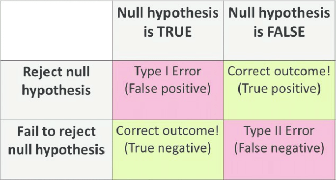
So Type I and type II error is one of the most important topics of hypothesis testing. Let’s simplify it by breaking down this topic into a smaller portion.

A false positive (type I error) — when you reject a true null hypothesis.
A false negative (type II error) — when you accept a false null hypothesis.
The probability of committing Type I error (False positive) is equal to the significance level or size of critical region α.
α= P [rejecting H0 when H0 is true]
The probability of committing Type II error (False negative) is equal to the beta β. It is called the ‘power of the test’.
β = P [not rejecting H0 when h1 is true]
Example:
The person is arrested on the charge of being guilty of burglary. A jury of judges has to decide guilty or not guilty.
H0: Person is innocent
H1: Person is guilty
Type I error will be if the Jury convicts the person [rejects H0] although the person was innocent [H0 is true].
Type II error will be the case when Jury released the person [Do not reject H0] although the person is guilty [H1 is true].
Statistically significant
To understand this topic let us consider an example: Suppose there is a candy bar factory which makes 500gm of candy bar every day. One day after the maintenance of the factory, one worker claims that they no more make 500gm of candy, it may be less or more. So on what basis did the worker claim this error??? So where do we draw a line to make a decision about the variation in the weight of candy bars? This decision/boundary is Statistically significant.
Level of confidence
As the name suggests a level of confidence: how confident are we in taking out decisions. LOC(Level of confidence) should be more than 95%. Less than 95% of confidence will not be accepted.
Level of significance(α)
The significance level, in the simplest of terms, is the threshold probability of incorrectly rejecting the null hypothesis when it is in fact true. This is also known as the type I error rate.
It is the probability of a type 1 error. It is also the size of the critical region.
Generally, strong control of α is desired and in tests, it is prefixed at very low levels like 0.05(5%) or 01(1%).
If H0 is not rejected at a significance level of 5%, then one can say that our null hypothesis is true with 95% assurance.
P-value
Let’s suppose we are conducting a hypothesis test at a significance level of 1%.
Where, H0: mean<X (we are just assuming a scenario of 1 tail test.)
We obtain our critical value (based on the type of test we are using) and find that our test statistic is greater than the critical value. So, we have to reject the null hypothesis here since it lies in the rejection region. Now if the null hypothesis is getting rejected at 1%, then for sure it will get rejected at the higher values of significance level, say 5% or 10%.
What if we take significance level lower than 1%, would we have to reject our hypothesis then also?
Yes, there might be a chance that the above scenario can happen, and here comes “p-value” in play.
the p-value is the smallest level of significance at which a null hypothesis can be rejected.
That’s why many tests nowadays give p-value and it is more preferred since it gives out more information than the critical value.
For right tailed test:
p-value = P[Test statistics >= observed value of the test statistic]
For left tailed test:
p-value = P[Test statistics <= observed value of the test statistic]
For two tailed test:
p-value = 2 * P[Test statistics >= |observed value of the test statistic|]
Decision making with p-value
We compare p-value to significance level(alpha) for taking a decision on Null Hypothesis.
If p-value is greater than alpha, we do not reject the null hypothesis.
If p-value is smaller than alpha, we reject the null hypothesis.
I hope this article clears some basic terms used in Hypothesis testing. But this is not the end. I will come up with Hypothesis testing techniques soon. Thank you so much for studying this blog. 🙂
About the Author
 Ritika Singh – Data Scientist
I am a Data scientist by profession and a Blogger by passion. I have been working on machine learning projects for more than 2 years. Here you will find articles on “Machine Learning, Statistics, Deep Learning, NLP and Artificial Intelligence”.


Hi, Thanks for the article. Can you give examples from the text in R? vlad
Dear, What if P value is equal to alpha?? Which hypothesis will be accepted null or alterative?? Regards, Shahroz Khan
Systematically Explained. #A great thanks to you Mm.