Introduction
In recent years, data science has become omnipresent in our daily lives, causing many data analysis tools to sprout and evolve for the data scientist Joe to use. Python, R, or KNIME Analytics Platform, are some of the most common tools. The innovative character of the KNIME Analytics Platform consists of its visual programming environment with an intuitive interface that embraces a wide variety of technologies.
In this blog post, we would like to give you a friendly introduction to the KNIME Analytics Platform, by showing you the user interface, explaining the most crucial functionalities, and demonstrating how to create a codeless data science process. In order to do that, we will use a specific example of implementing a workflow for customer segmentation based on the k-Means clustering procedure.
General Concepts: Nodes, Workflows, & Components
KNIME Analytics Platform is a free, open-source software for the entire data science life cycle. KNIME’s visual programming environment provides the tools to not only access, transform, and clean data but also train algorithms, perform deep learning, create interactive visualizations, and more.
The KNIME Analytics Platform user interface also referred to as workbench, is typically organized as shown in Fig. 1.
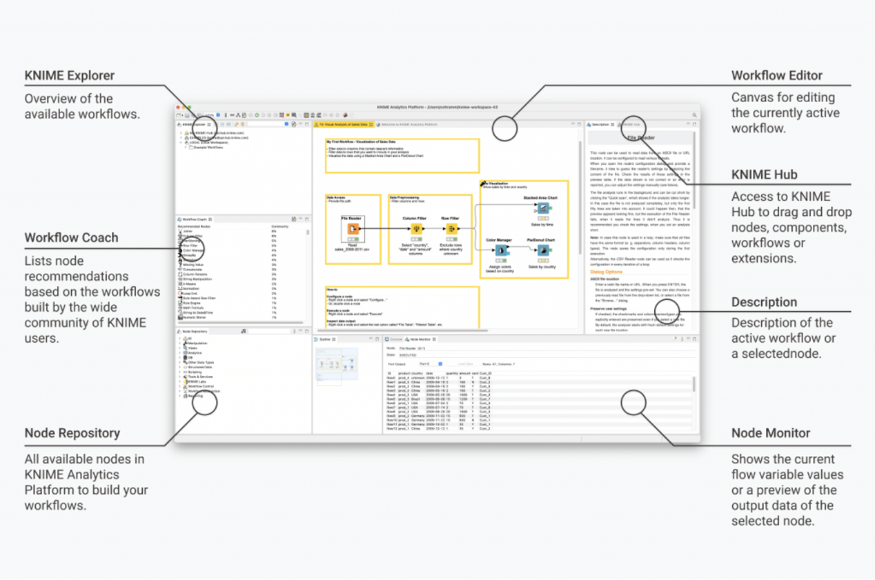
Nodes perform tasks in your data science process.
When you are assembling a visual workflow, you will be using “nodes”. A node is displayed as a colored box and performs an individual task. A collection of interconnected nodes is your assembled workflow and represents some part – or all – of your data analysis project.
Each node can perform all kinds of tasks, e.g., reading and writing files, transforming data, training models, or creating visualizations. All the different types of nodes are found in the Node Repository (in the lower-left corner). The data are routed through the node via input and output ports. A node can have data as input or output as well as other objects, such as connections or machine learning models, SQL queries, or data properties. Each object inputs or outputs the node via a dedicated port. Only ports of the same type can be connected. Nodes are color-coded, according to their category, e.g., all yellow nodes are for data wrangling. Depending on their task, nodes also have specific settings, which can be adjusted in their configuration dialog.
A simple traffic light system underneath each node shows you whether the node is already configured, executed, or whether an error has occurred.
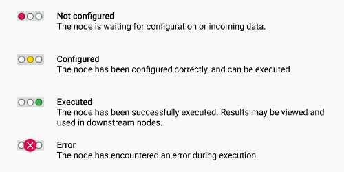
Figure 2. The different states of a node
Workflows are assembled with nodes, metanodes, and components.
A workflow in KNIME Analytics Platform consists of several, combined nodes. The data flows through the workflow from left to right through the node connections.
You can use a so-called annotation – a colored frame that can be placed freely inside a workflow – to document the steps in your workflow.
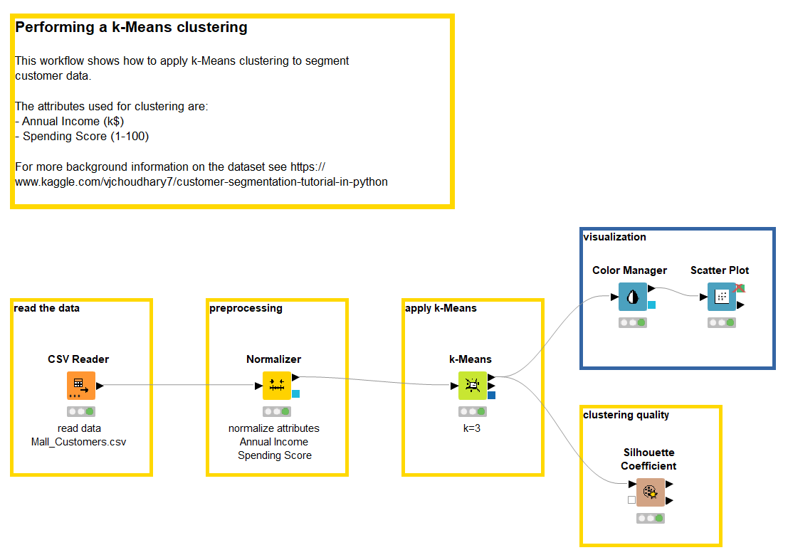
Figure 3. A simple workflow performing customer segmentation through a k-Means clustering procedure. The workflow’s task as well as each step- read the data – preprocessing – apply k-Means – visualization – is documented inside annotation boxes.
You can also identify isolated blocks of logical operations in your workflows and include these nodes into so-called metanodes or components. Components are like metanodes but instead of just grouping some nodes for the sake of transparency, they encapsulate and abstract the functionalities of the logical block. Components serve a similar purpose as nodes, whereas a metanode is more of a visual appearance improvement.
Enrich functionality with extensions and integrations and utilize resources
Aside from all the above-mentioned functions, the KNIME Analytics Platform has two further important elements – extensions and integrations. The variety of extensions and integrations provide additional functionalities to the KNIME core functions. For example, the KNIME Deep Learning – Keras Integration or the Text Processing extension are only two of many exciting possibilities.
Finally, just a few words on where to get help and find resources.
The KNIME Hub is a public repository, where you can find vast amounts of nodes, components, workflows, and extensions and provides a space to collaborate with other KNIME users. On KNIME Hub, you can find example workflows and pre-packaged components to get started.
The KNIME Community Forum serves as an environment to exchange experiences with other KNIME users, to seek help, or to offer your skills to help others.
If you need help getting started, on our Learning webpages you will find additional courses and material.
The Example: Customer Segmentation
Let’s now put our knowledge into practice and assemble a visual workflow in which a k-Means clustering is applied to segment customer data.
The dataset we use for this example can be downloaded from Kaggle and contains some basic customer data: “Customer ID”, “Gender”, “Age”, “Annual Income”, and “Spending Score”.
There are many ways to perform customer segmentation. Most of them include some previous knowledge on at least one of the input attributes. When nothing is known, in terms of knowledge or goals, customer segmentation is often performed via a clustering technique.
In general, clustering is used to detect underlying patterns in the data. Similar traits – or data points – are grouped together based on similarity and assigned into clusters. Amongst all clustering techniques, k-Means is a very simple one, yet effective enough.
Let’s now implement a workflow that reads the data, applies the k-Means algorithm, evaluates the quality of the final clustering, and visualizes the obtained cluster set. This workflow is shown in Fig. 3 and can be downloaded for free from the KNIME Hub.
a) Read the Dataset with CSV Reader
First, you need to read your data into the workflow. KNIME Analytics Platform offers a variety of data reading options for different file types, for example, Excel files with the Excel Reader node, text files with the File Reader node, or CSV files with the CSV Reader node. It is also possible to connect to and read from a database using the dedicated DB nodes. To read your data into KNIME Analytics Platform there are two different options.
You can drag and drop your file into the workflow. In this case, if it is a known file extension, the KNIME Analytics Platform automatically creates the correct reader node and automatically feeds the file location into the node configuration settings.
Alternatively, you can create and configure the node manually. Select the corresponding reader node (Fig. 4) from the Node Repository, drag & drop it into the workflow editor area, double-click the newly created node (or right-click and then select “Configure”), and insert the file location in the configuration window.
The configuration window of the CSV Reader node (Fig. 5) shows a preview of the data to be read. Here, we can spot reading problems, if any, and fix them appropriately in this same configuration window. If the data seem to be read correctly, then we just click “OK” in the lower right corner of the node configuration window.
Note that those are standard operations.
- To create a node, you locate it in the Node Repository and double-click it or drag & drop it into the workflow editor area. The node is then created with a red traffic light status.
- To configure the node, double-click it (or right-click it and select “Configure”), adjust the settings appropriately, and then click the button “OK” to save them. The traffic light changes to yellow.
- To execute a node, right-click it and select “Execute” or select it and then click the green single arrowed button in the toolbar.
- To display the node results, right-click the node and select the last option in the context menu.
In our case, we located the file Mall_Customers.csv and dragged and dropped it into the Workflow Editor in the center of the KNIME Analytics Platform workbench. The CSV Reader node was automatically created, and the node dialog opened with the settings automatically filled in (Fig. 5). In this case, all settings are correct, we just click “OK” at the bottom of the configuration window.
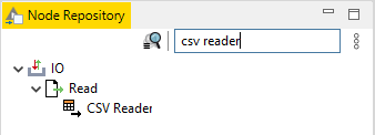
Figure 4. Searching the CSV Reader node via Node Repository
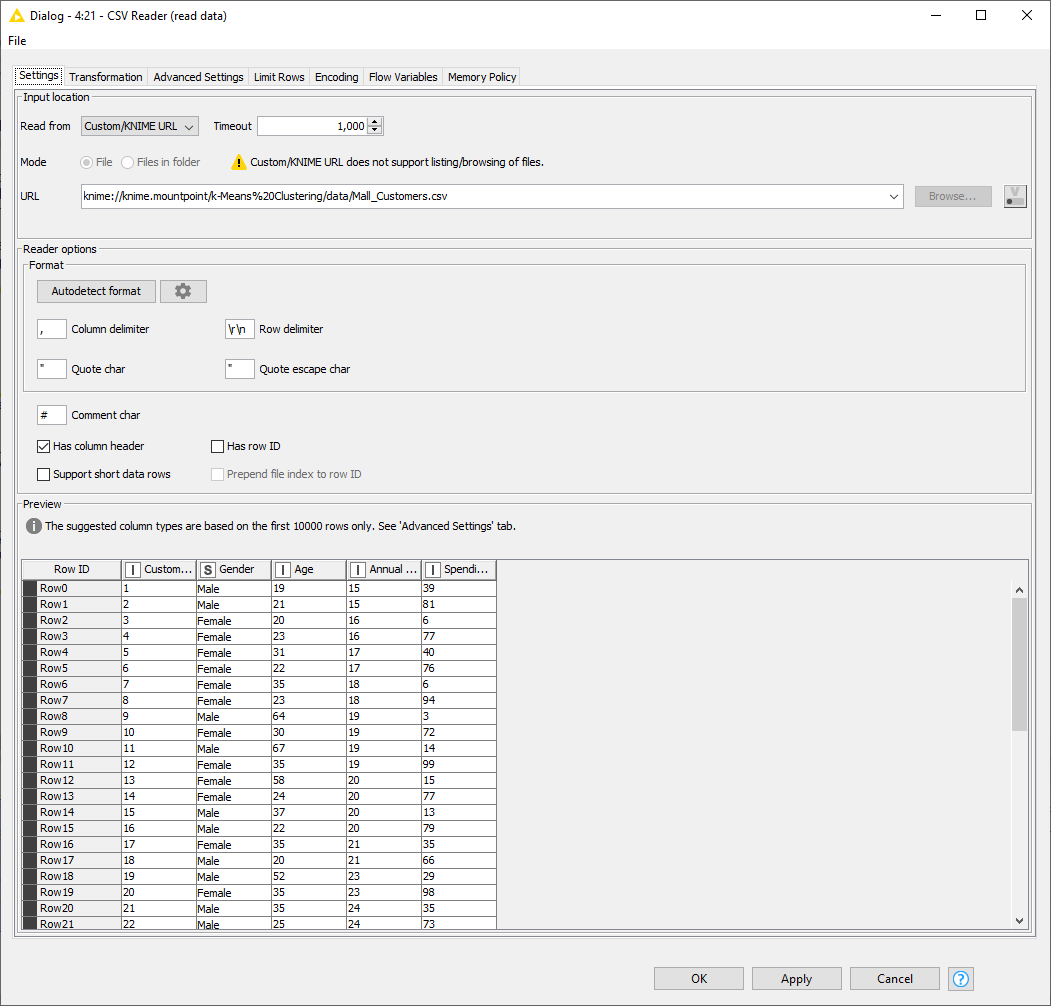
Figure 5. The configuration window of the CSV Reader node.
b) Apply Normalization to Attributes with Normalizer Node
The k-Means algorithm requires normalized numerical attributes. In general, normalization is necessary, when the attributes are in two different non-comparable units (e.g., cm and kg) or the variance between attributes is quite different. By normalizing the values, we make sure that one input feature does not dominate the other features in the distance or variance calculation. Additionally, nominal attributes should be discretized before feeding them into the algorithm, otherwise, it cannot handle them properly. Discretize nominal variables using the Category to Number node.
Our dataset consists of five attributes, of which one is a categorical variable (“Gender”), and the other four are numerical variables. Usually, the best practice is to use all input attributes, but in this case, we decided to limit ourselves to just two: Annual Income and Spending Score. We did this to obtain a clearer visualization of the results in a 2D scatter plot and thus an easier comparison of different k-Means runs.
In the configuration window of the Normalizer node (Fig. 6), you need to select the attributes for which normalization is required. We decided to use a min-max normalization to simply transform the values into a [0,1] interval, where the smallest value is transferred to 0 and the largest value to 1. But of course, there are other options, like a z-score normalization (suitable when having many outliers) or normalization by decimal scaling.
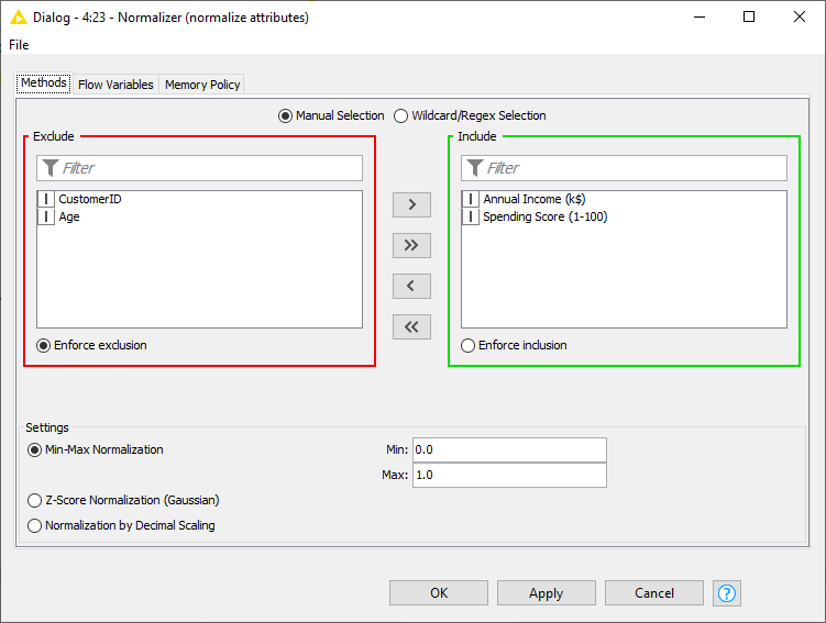
Figure 6. The configuration window of the Normalizer node.
We insert the Normalizer node (by drag & drop or double click).
To connect two nodes, right-click the output port of node A and drag the cursor to the input port of node B. Alternatively, select node A and double-click node B in the Node Repository: this will automatically create node B and automatically connect it to selected node A.
We then configure the Normalizer node appropriately (Fig. 6).
Nodes can either be executed step by step to examine intermediate results or the entire workflow at once. The two green arrowed buttons in the toolbar are responsible for these two types of execution.
c) Apply k-Means Algorithm and Configure Cluster Number
Now, connect the normalized dataset to the k-Means node and configure the number of clusters k. The correct choice of a number of clusters cannot be known beforehand. Usually, a few numbers clusters are tried and then the final cluster sets are visually compared and evaluated. Alternatively, the quality of the different cluster sets can be measured and compared, for example via the Silhouette Coefficient. The optimal k could also be obtained by running an optimization method, like the elbow method, the Silhouette optimization, or the Gap Statistics.
Let’s start with k=3. In the node configuration window of the k-Means node (Fig. 7), we can decide whether to initialize the algorithm with the first k rows or with k random data points of the dataset. Also, we can include or exclude attributes for the distance calculation.
You might now wonder why there is no option for the distance measure. In this case, let me point out that the k-Means node uses the Euclidean distance by default. Notice that the Euclidean distance only applies to numerical attributes and therefore only numerical columns are available to move from the Include to the Exclude panel and vice versa. We use the two normalized input attributes Annual Income and Spending Score. Would we obtain the same results when adding attribute Age? You can try…
The configuration window also includes an emergency stop criterion, to avoid infinite running without convergence to a stable solution. This is the setting named Max. Number of Iterations.
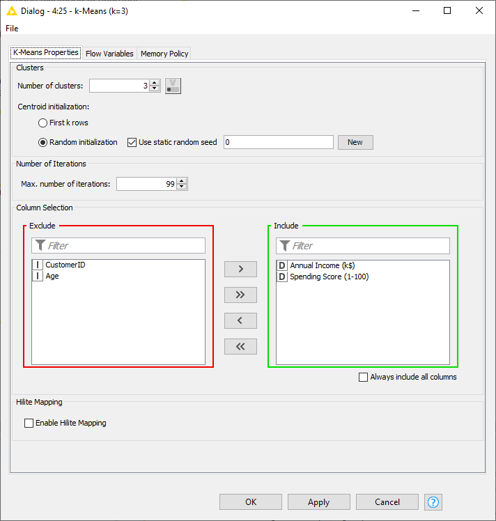
Figure 7. The configuration window of the k-Means node.
After executing this node successfully, it outputs the k cluster centers for the k=3 clusters (Fig. 8). You can try to run the algorithm again with a different number of clusters and see if and how the cluster centers change.
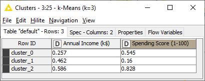
Figure 8. The three cluster centers.
d) Determine Clustering Quality with Silhouette Coefficient
Now we successfully identified three clusters. But how good is our clustering? More precisely, how good is the choice of our k? The quality of the cluster set can be measured via the Silhouette Coefficient as calculated via the Silhouette Coefficient node.
As in the k-Means node, an Include/Exclude panel allows to include attributes for the calculation of the Silhouette Coefficient. In addition, here, the cluster column must be selected, which in our case comes from the previous k-Means node, is called “Cluster”, and contains a string value indicating the cluster affiliation.
When the node is successfully executed, you can right-click it and investigate either the table, where for each tuple the cluster affiliation and the Silhouette Coefficient is displayed or the table where the mean Silhouette Coefficient is reported for each cluster together with the overall mean value. In our case, the overall mean Silhouette Coefficient is 0.45, which is not too bad but there is still room for improvement. Let’s try different values for k and see if better clustering can be achieved.
e) Assign Color to Clusters with Visualization Nodes, Color Manager & Scatter Plot
The last step refers to visualizing the obtained clusters. To do so, we use the Color Manager node to assign a specific color to each cluster (Fig. 9) and after that the Scatter Plot node to visualize the resulting cluster set (Fig. 10). Indeed, a visual inspection can help us evaluate the quality of the cluster set.
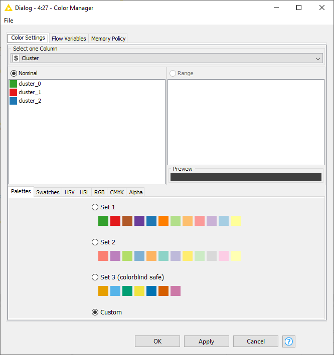
Figure 9. The configuration window of the Color Manager node.
In Fig. 10, you see the configuration window for the Scatter Plot node and its most important setting: selecting attributes for the x and y axis. In the tab “General Plot Options”, chart title and subtitle can be specified.
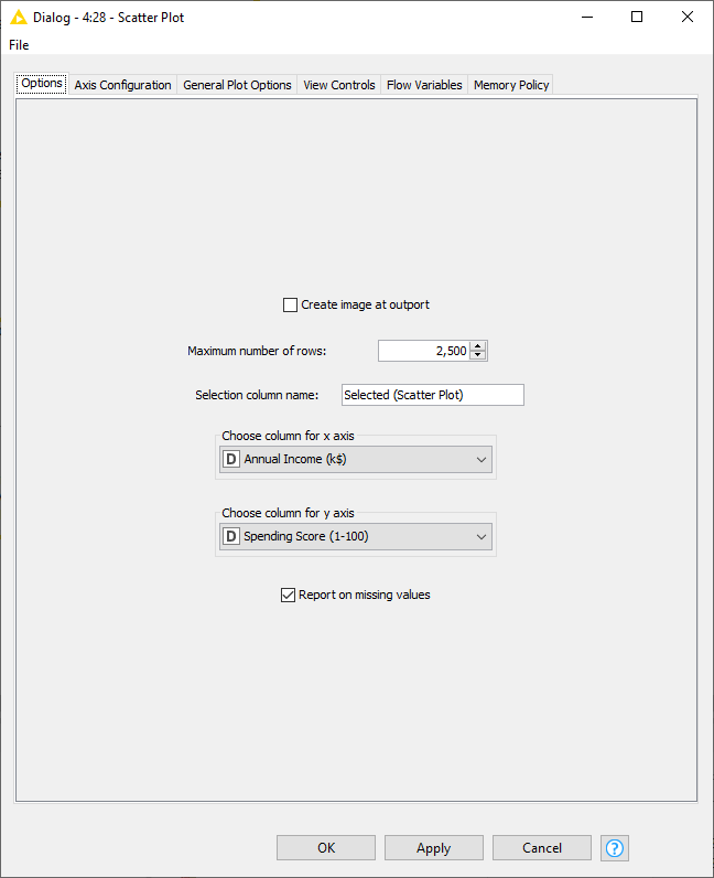
Figure 10. The configuration window of the Scatter Plot node.
Now, let’s look at the visualization (Fig. 11). As you can see, the clusters are quite widespread, especially cluster 0 and cluster 1. This and the Silhouette Coefficient of 0.45 indicates that we might need to rethink our parameter choice.
f) Document Workflow with Comments and Annotations
Let’s now add a few comments into the workflow.
To insert an annotation, right-click anywhere in the workflow and click “New Workflow Annotation”. You can then edit the color, frame width, and font by double-clicking the top left corner of the square. Inside the annotation, you can then write some description about the task implemented by the workflow or parts of the workflow.
The final workflow is shown in Fig. 3 and can be downloaded from the KNIME Hub.
Try Out Different k’s
In case the clustering is not as satisfying as expected, simply rerun k-Means with different parameters and see if a better clustering can be achieved.
Below, we report the mean Silhouette Coefficient for k=3, k=5, and k=8 and the corresponding scatter plots.
Table 1. The mean overall Silhouette Coefficient for different k
| k=3 | k=5 | k=8 | |
| Overall Silhouette Coefficient | 0.45 | 0.56 | 0.44 |
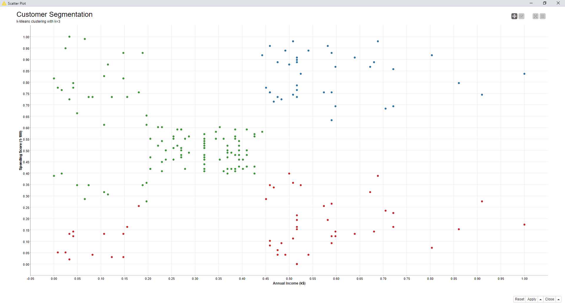
Figure 11. The visualization of the resulting cluster set for k=3.
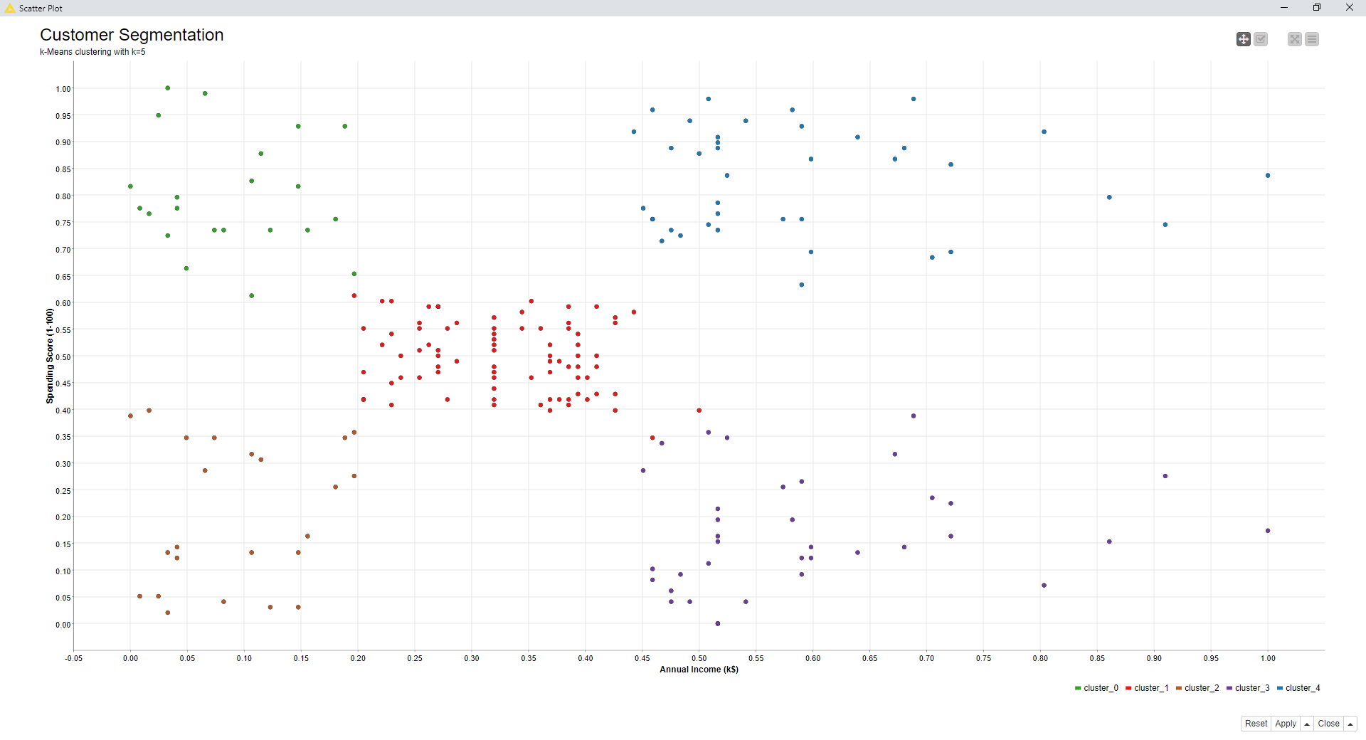
Figure 12. Cluster set for k=5
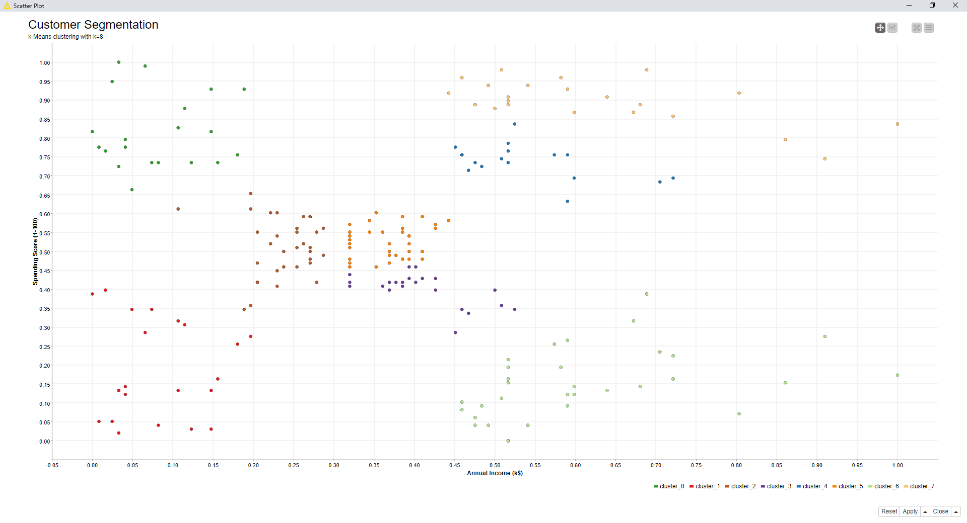
Figure 13. Cluster set for k=8
By comparing the scatter plots (visually) and the silhouette coefficient values, k=5 seems to be the preferable choice, so far. However, using the optimization procedure based on the Silhouette Coefficient and implemented in the component named “Optimized k-Means (Silhouette Coefficient)”, k=5 turns out to be the best choice for setting k.
Now, we should explain how to create and use a component… but this is material for the next article.
The media shown in this article are not owned by Analytics Vidhya and is used at the Author’s discretion.


This guide is incredibly helpful for someone just starting with KNIME! The step-by-step approach makes it easy to follow along, and I appreciate the clear explanations of the different nodes. Looking forward to experimenting with these techniques in my own projects!