What is Machine Learning?
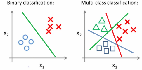
Machine Learning is a popular topic in Information Technology in the present day. Machine Learning allows our computer to gain insight from data and experience just as a human being would. In Machine Learning, programmers teach the computer how to use its past experiences with different entities to perform better in future scenarios.
Machine Learning involves constructing mathematical models to help us understand the data at hand. Once these models have been fitted to previously seen data, they can be used to predict newly observed data.
In Machine Learning, models are only as useful as their quality of predictions; hence, fundamentally our goal is not to create models but to create high-quality models with promising predictive power. We shall now examine strategies for evaluating the quality of models that are generated by our Machine Learning Algorithms.

Source: Nokia Corporation.
Evaluating Binary Classifier Predictions.
When it comes to evaluating a Binary Classifier, Accuracy is a well-known performance metric that is used to tell a strong classification model from one that is weak. Accuracy is, simply put, the total proportion of observations that have been correctly predicted. There are four (4) main components that comprise the mathematical formula for calculating Accuracy, viz. TP, TN, FP, FN, and these components grant us the ability to explore other ML Model Evaluation Metrics. The formula for calculating accuracy is as follows:

Source: My PC
Where:
- TP represents the number of True Positives. This refers to the total number of observations that belong to the positive class and have been predicted correctly.
- TN represents the number of True Negatives. This is the total number of observations that belong to the negative class and have been predicted correctly.
- FP is the number of False Positives. It is also known as a Type 1 Error. This is the total number of observations that have been predicted to belong to the positive class, but instead, actually, belong to the negative class.
- FN is the number of False Negatives. It may be
referred to as a Type 2 Error. This is the total number of observations that
have been predicted to be a part of the negative class but instead belong to
the positive class.
The main reason for individuals to utilize the Accuracy Evaluation Metric is for ease of use. This Evaluation Metric has a simple approach and explanation. It is, as discussed before, simply the total proportion (total number) of observations that have been predicted correctly. Accuracy, however, is an Evaluation Metric that does not perform well when the presence of imbalanced classes-when in the presence of imbalanced classes, Accuracy suffers from a paradox; i.e., where the Accuracy value is high but the model lacks predictive power and most, if not all, predictions are going to be incorrect.
For the above reason, when we are unable to use the Accuracy Evaluation Metric, we are compelled to turn to other evaluation metrics in the scikit-learn arsenal. These include, but are not limited to, the following Evaluation Metrics:
Precision
This refers to the proportion (total number) of all observations that have been predicted to belong to the positive class and are actually positive. The formula for Precision Evaluation Metric is as follows:

Source: My PC
Recall
This is the proportion of observation predicted to belong to the positive class, that truly belongs to the positive class. It indirectly tells us the model’s ability to randomly identify an observation that belongs to the positive class. The formula for Recall is as follows:

Source: My PC
F1 Score.
This is an averaging Evaluation Metric that is used to generate a ratio. The F1 Score is also known as the Harmonic Mean of the precision and recall Evaluation Metrics. This Evaluation Metric is a measure of overall correctness that our model has achieved in a positive prediction environment-
i.e., Of all observations that our model has labeled as positive, how many of these observations are actually positive. The formula for the F1 Score
Evaluation Metric is as follows:
![]()
Source: My PC
Evaluating Multiclass Classifier Predictions.
As we have learned from earlier information in the article, in Machine Learning, all input data is not balanced, hence the issue of Imbalanced Classes. With the Accuracy Evaluation Metric removed from our options, we specifically turn to Precision, Recall, and F1 Scores. We use parameter
options in Python, which are used for aggregating the evaluation values by averaging them. The three main options that we have available to us are:
- _macro – Here we specify to the compiler to calculate the mean of metric scores for each class in the dataset, weighting each class equally.
- _weighted – We calculate the mean of metric scores for each class, and we weigh each class directly proportional to its size in the dataset.
- _micro – Here we calculate the mean of metric
scores for each OBSERVATION in the dataset.

Source: Medium.
Visualizing a Classifier’s Performance.
Currently, the most popular way to visualize a classifier’s performance is through a Confusion Matrix. A Confusion Matrix may be referred to as an Error Matrix. A Confusion Matrix has a high level of interpretability. It comprises a simple tabular format, which is often generated and visualized as a Heatmap. Each Column of the Confusion Matrix represents the predicted classes, while every row shows the true (or actual) classes.
There are three important facts to be aware of about a Confusion Matrix:
- A Perfect Confusion Matrix will have values along the main diagonal (from left to right), and there will zeroes (0) everywhere else in the confusion matrix.
- A Confusion Matrix does not only show us where the Machine Learning Model faltered but also how it reached those conclusions.
- A Confusion Matrix will function with any number
of classes, i.e., Having a dataset containing 50 classes, will not affect model
performance nor the Confusion Matrix- it just means your Visualized Matrix will
be very large in size.

Source: ResearchGate.
Evaluating a Regression Model’s Performance.
For a Regressor, you will find that one of the most used and well-known Evaluation Metrics is MSE. MSE stands for Mean Squared Error. Put into a mathematical representation, MSE is calculated as follows:
Source: My PC.
Where:
- n represents the number of observations in the dataset.
- yi is the true value of the target value we are trying to predict for observation I.
- ŷi is the model’s predicted value for yi.
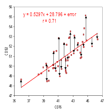
MSE is a calculation that involves finding the squared sum of all the distances between predicted and true values. The higher the output value for MSE, the greater the sum of squared error present in the model, and hence, the worse the quality of model predictions. There are advantages of squaring the error margins, as seen in the model:
- Firstly, squaring the error constrains all error values to be positive.
- Secondly, this means the model will penalize few
large error values, more than it will penalize many small error values.

Source: Statistics How To.
This concludes my article on Machine Learning Model Evaluation.
Thank you for your time.
The media shown in this article are not owned by Analytics Vidhya and is used at the Author’s discretion.


