Introduction
Hadoop is the most commonly perceived word when coming to Big Data Technology. The above image shows the various tool and technologies used in Hadoop Framework.
Hadoop is not a programming language instead, Hadoop is a framework which consists of various tool and technologies for data storage and data processing.
Hadoop Features
Big Data is involved with handling the humungous amount of data. Hadoop acts as a catalyst for manipulating this data. Data – Processing layer is handled by MapReduce or Spark or a combination of both. The Data Storage layer is handled by HDFS mainly, others involve HIVE and HBase.
1) HDFS Storage Layer –
This is the base of the Hadoop Framework. HDFS stores all types of data – Structured, Semi-Structured, Unstructured Data.
2) Hive Storage Layer –
Hive replicates the RDBMS (Relational Database Management Systems). Thus it stores Structured Data in table format.
3) HBase Storage Layer –
Since HBase is a NO-SQL database, it satisfies the property of handling both unstructured data and semi-structured data.
In this article, we will cover all topics related to HIVE STORAGE STRUCTURE. Before proceeding to it, let’s have a look at the comparisons between different types of data.
Classification of Data into 3 major types
Different Types of Data
Data is instead content that we consume in a day to day life. Be it an uninterrupted amount of time we scroll through Facebook or any other social forums. Data comes in different sizes and shapes. Is storing the data important?? How can this data provide value to us??
Imagine If you are a startup owner of an offline retail brand mainly focusing on women’s wear and have a strong urge to hit it online. You need to increase the brand visibility online through all social channels.
Let’s take Facebook as an example to scale your business. To build your brand you need to pinpoint your target audience. The target audience generates leads in return thus generating prospects or customers. These leads are generated mostly by Facebook ads.
But to run ads, you need to analyze who your customers are!! The likes and dislikes are based on the type of content they are consuming on Facebook. It’s like from a sea full of fishes, you choose to fish and grab Pomfret that will satisfy your taste bud.
So, this analysis of human behavior based on content will drive your business to earn bountiful profits. Thus, data is extremely more important.
This content/data is split up into different formats:-
1) Structured Data:–
Data in table format structure.
An Example of Relational Database
Here the data is stored in row and column format. It rules on the concept of schema on write. Schema on write states that “Before entering the data into the storage system/database fields are validated and then stored into the system.” Thus the read becomes quite easier.
2) Unstructured Data:-
Data that does not have a relational structure.
Different data formats that come under Unstructured Data
It cannot be stored as tables i.e. rows and columns. It rules on the concept of schema on reading. Schema on read states that “Before storing the data no validation is required you can dump the data and then while querying/fetching the data proper structure is given to the data. ” Thus, writing becomes easier as we can store any type of data. Example:- HIVE
3) Semi-Structured Data:-
An unstructured data but has a structure towards it.
JSON format structure
Eg of such data includes JSON files or XML files. Let’s take the above example.
a) Employees:- defines the table structure.
b) first name, last name – define the column names of the employee’s table
c) John, Anna, Peter – column values for column firstName.
HIVE STORAGE STRUCTURE
In this article, we will cover:-
· Installation of Cloudera to access hive storage
· Types of Tables in Hive
· DDL, DML commands
· 2 types of Partitioning
· Bucketing
A) HIVE:-
A hive is an ETL tool. It extracts the data from different sources mainly HDFS. Transformation is done to gather the data that is needed only and loaded into tables.
Hive acts as an excellent storage tool for Hadoop Framework. Hive is the replica of relational management tables. That means it stores structured data. However, Hive can also store unstructured data. Hive firstly loads the unstructured data from HDFS, creates a structure around it, and loads the data.
B) Installing Cloudera to built a Hive storage system on top of HDFS:-
Cloudera is an open-source data platform through which we can access all Hadoop tools and technologies.
The below link will help in installing Cloudera in your respective machines –
https://www.youtube.com/watch?v=L3KFoq3Snt8&t=122s
After installing Cloudera, you will see a VDI screen open.
On the Desktop shown above, there is a logo of Cloudera Enterprise Express Trial.

By clicking on the logo will automatically load a terminal as shown below.
Open a new terminal and execute the command given in the below terminal. It will start the Cloudera Manager and we can access the services of the Hadoop framework via http://quickstart.cloudera:7180
Paste the http://quickstart.cloudera:7180 URL given in the VMware browser and enter the username and password to access the Cloudera Manager via browser.
Once you log in, on the left-hand side you will see a list of all services that the Hadoop framework serves.
Important:-
You don’t need to start all the services as it will result in a huge network I/O. It’s always recommended to start those services which you need at a given point in time. For Eg., we need a HIVE storage structure, so along with that, we need to start HDFS service as well. Else you will encounter an error when you log in to hive through the terminal. The reason behind Hive sits on top of HDFS. So whatever data you store in HIVE, the metadata and the data itself get stored in the HDFS directory.
The above image shows how we can start the services in Cloudera Manager. Once we start the HDFS and HIVE service successfully, we can open a new terminal and log in to the hive.
The above image shows that you have logged into the hive terminal !!
A) Hive supports 2 types of tables:-
Hive stores the data into 2 different types of tables according to the need of the user.
a) Internal Table/Managed Table:-
Managed Table is nothing but a simply create table statement. However, this is the default database of HIVE. All the data that is loaded is by default stored in the/user/hive/warehouse directory of HDFS.
Once the table is deleted or dropped, there is no way to retrieve it because the data and its metadata get completely vanished.
b) External Table:-
External table is created by using the keyword external in the create table statement. The location of the external table is not the same as that of the managed table. External tables are those whose metadata gets deleted however table data gets preserved in the directory.
DDL operations like Drop, Truncate cannot be directly executed on an external table. You have to change the status of the table as internal or managed to do so.
B) DDL and DML commands based on Managed/External Tables:-
a) Database creation
You can create a database in whichever format you like. Here, I have created a database in 3 ways.
For creating a database at the location you desire, you need to create a directory in HDFS and then create a database and include the location of the newly created path in DBPROPERTIES.
Here, in the below screenshot, a database employee_db is created with the location as ‘/user/hive/new_location’.
You can verify the output by logging into quickstart.cloudera:50070/explorer.html Here in the below screenshot, you will find the directory as new_location
You can always verify the output through the terminal as well.
The above screenshot shows creating the database by validating whether the database is present in the system or not. If it is not present, the database will get created else it will be thrown an error as ‘Database db_name already exists’
b) Get a list of databases present in the system
c) Using a particular database and accessing the tables from within
Here, in this case, you can either execute the command use database_name, or while accessing tables you can directly execute as database_name.table_name
d) Pattern Matching to retrieve the database you need
Suppose you have millions of databases but you don’t remember the exact name of the database, you can use pattern matching to retrieve the database you require.
e) To get complete information of a database
Here, you get information related to a database like the location where the database is located, etc.
f) Table creation in Managed
Here, a normal table or managed table is created without any additional keyword.
· Ways to check whether the table is managed or external
Using the command describe formatted table_name, you will get information about the Table Type, column names and its data type, and the rest of the properties.
· Inserting the data into the table by 3 methods:-
We can insert the data into the tables via 3 formats:-
Load data inpath:– It means the data is already present in the HDFS path. The data is loaded from HDFS directly to the hive tables.
Load data local inpath:- means the data which is in different formats(parquet, orc, CSV, etc) is loaded from the local machine to tables in the hive. Local Machine means in simple terms File Explorer where you store all the files in different folders.
In the above screenshot, we have executed using the keyword local. This means the text file named student is present in the local directory and is loaded into table student.
The data loaded in the hive database is stored at the HDFS path – /user/hive/warehouse. If the location is not specified, by default all metadata gets stored in this path.
In the HDFS path, the data is stored in blocks of size either 64 or 128 MB. Here as you can see the data is stored at Block 0.
g) Table creation in External table format
An external table should be created always with the keyword external in it.
· Creating an external table
· Loading the data into an external table same as loading in the managed table
· Description of the external table using describe command
Here Table_Type is given as External Table.
h) Drop table command in External Table
Drop table command is simple with that of Managed tables. But in the external table, it’s impossible to drop the table with the command drop table table_name
The below screenshot shows an attempt to drop an external database.
To drop an external table, we need to alter or change the definition of a table from external to managed.
Thus, by changing the external table to managed table we can drop the database. Also, it follows a pattern such as first drop the table and then database irrespective of any tables.
i) Alter table commands for both types of tables
Alter table involves – Addition of a column to an existing table
– Renaming the table
– Changing the column names
– Drop unwanted columns
· Renaming the table
· Addition of columns to an existing table
· Renaming the existing column name to a new one
· Drop unwanted columns
Here, we use replace command with all the required fields in it, thus automatically it drops the columns you don’t require.
Here, we dropped the column named Course.
E) Partitioning and its types:-
Partitioning in a hive table is equal to dividing the table based on the column values. The advantage of partitioning is that data is stored in slices and thus whenever a query is fired from millions of records, query response time becomes faster. Since values are fetched based on partitions, the query is executed in a matter of seconds.
If the partitioning concept didn’t exist, there would be a tremendous degradation of the performance of the query.
The partitioning in Hive can be executed in 2 main ways:-
· Static Partitioning:-
In static or manual partitioning, it is required to pass the values of partitioned columns manually while loading the data into the table. Hence, the data file doesn’t contain the partitioned columns.
First, select the database you need to create a static partitioned table
Create a Static Partitioned Table
Describe the table to see the partitions are created properly
Loading the data into respective partitions
In Static Partitioning, the data is divided according to the partitions and then stored as separate files in the local machine. For Eg., in the below screenshot, we have first loaded the file where Course = ‘ComputerEngineering’ and stored it as a student.txt file in the local machine. Then again repeated the same process where we loaded the file with Course = ‘Doctor’ and stored it as a separate text file as student1.txt.


Here, in the below screenshot, we can see partition being created according to different values of the columns we tend to partition.
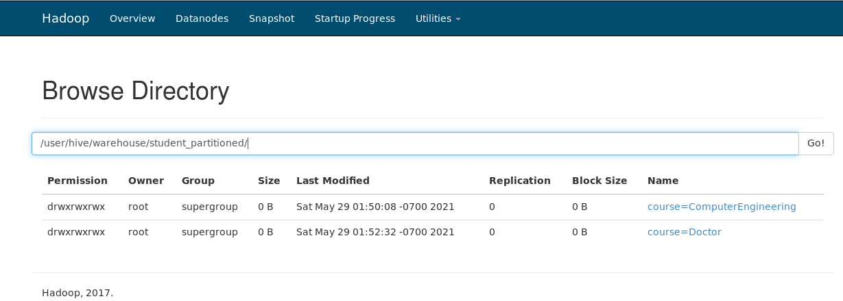
Thus, Static Partitioning is a type of partitioning where we manually create all partitions when loading the data.
· Creating a Dynamic Partitioned
First, create a new database or use an existing database to create dynamic partitioning.

In the below screenshot, non-strict means the partition applied to the table is dynamic(no manual work).


Now, create a normal table without partitions.

Load the entire data (not separate as student.txt, student1.txt as seen in static partitioning) into the table.

Now create a partitioned table as shown below.

load the data from the student table i.e. the normal table to the partition table(that’s where it is dynamic).
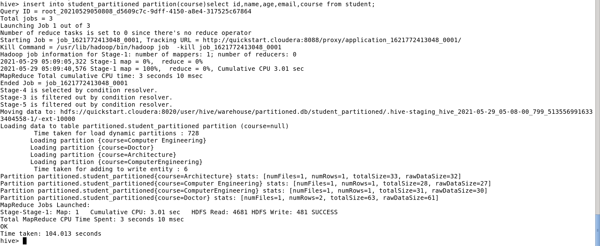
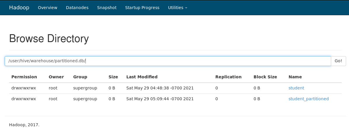
Now, when you browse the file system, you can see 2 tables. Student(normal table) and student_partitioned(Dynamic Partitioned table).
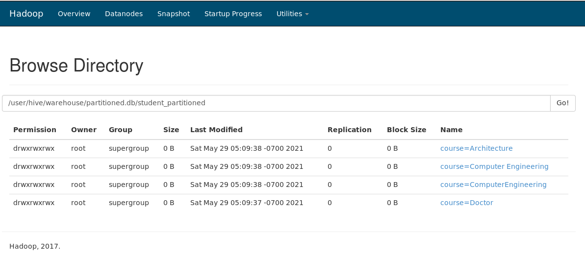
In the partitioned table, you will see all the partitions were included automatically based on the column we decided to partition. Here we have 4 partitions defined for column Course. That means it could find only those 4 values in the data file that we loaded in the table.
F) Bucketing in Hive
Bucketing is another data organizing technique in Hive. The same column values will go to the same bucket. Bucketing can be used separately or with partition. The concept of bucketing is based on the hashing technique. Here, modules of the current column value and the number of required buckets are calculated (let say, F(x) % 3). Now, based on the resulted value, the data is stored in the corresponding bucket.
First, as always use or create a database.


Create a normal table. Here in the below screenshot, a normal table called student is created.

Load the data into the table. Here, we have loaded the data named student.txt into table student.

By default, bucketing is kept to false. So we need to enable bucketing as shown below.

Now we create a bucketing table. Always remember when partitioning based on the column name, the column name is not included in create table statement but in bucketing the column name is included in create table statement and also in the bucketing keyword. We can explicitly set the number of buckets during table creation.
Bucketed Map Joins are the fastest joins – thus optimizing the hive. The rule for bucketed joins is – Both joining tables should be bucketed on the same columns as joining columns and both tables should have equal no of buckets.

Now load the data from the normal student table to bucketed table i.e. student_bucket
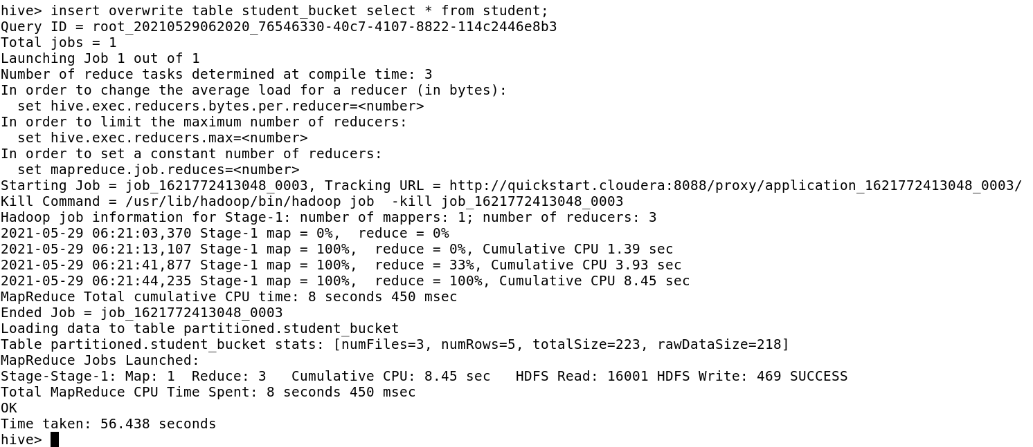
Now, as we notice in the file directory, there are 3 buckets(physical files) and data present in those files. Each file is stored in HDFS of block size 128 MB.
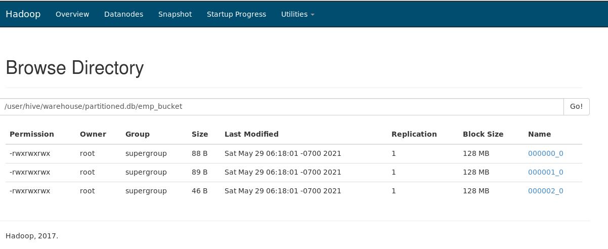
Thus, Partition and Bucketing can optimize the data present in Hive. HIVE can become a catalyst for handling all the operations concerning Hadoop Framework.
The media shown in this article are not owned by Analytics Vidhya and are used at the Author’s discretion.


