This article was published as a part of the Data Science Blogathon
Introduction
This article aims to explain Convolutional Neural Network and how to Build CNN using the TensorFlow Keras library. This article will discuss the following topics.
Let’s first discuss Convolutional Neural Network.
Convolutional Neural Network (CNN)
Deep learning is a very significant subset of machine learning because of its high performance across various domains. Convolutional Neural Network (CNN), is a powerful image processing deep learning type often using in computer vision that comprises an image and video recognition along with a recommender system and natural language processing ( NLP).
CNN uses a multilayer system consists of the input layer, output layer, and a hidden layer that comprises multiple convolutional layers, pooling layers, fully connected layers. We will discuss all layers in the next section of the article while explaining the building of CNN.
Let’s discuss the building of CNN using the Keras library along with an explanation of the working of CNN.
Building of CNN
We will use the Malaria Cell Image dataset. This dataset consists of 27,558 images of microscopic blood samples. The dataset consists of 2 folders – folders-Parasitized and Uninfected. Sample Images-
a) parasitized blood sample
b) Uninfected blood sample
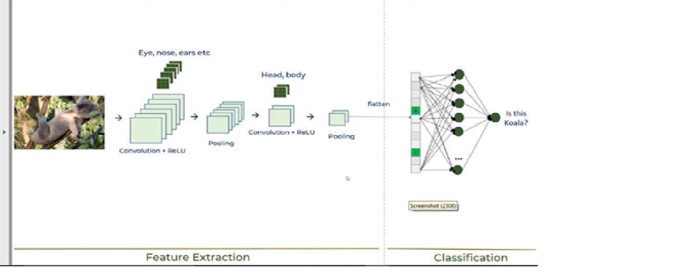
We will discuss the building of CNN along with CNN working in following 6 steps –
Step1 – Import Required libraries
Step2 – Initializing CNN & add a convolutional layer
Step3 – Pooling operation
Step4 – Add two convolutional layers
Step5 – Flattening operation
Step6 – Fully connected layer & output layer
These 6 steps will explain the working of CNN, which is shown in the below image –
Now, let’s discuss each step –
1. Import Required libraries
Kindly refer to the below link for detailed explanations of Keras modules.
https://keras.io/getting_started/
Python Code :
from tensorflow.keras.layers import Input, Lambda, Dense, Flatten,Conv2D
from tensorflow.keras.models import Model
from tensorflow.keras.applications.vgg19 import VGG19
from tensorflow.keras.applications.resnet50 import preprocess_input
from tensorflow.keras.preprocessing import image
from tensorflow.keras.preprocessing.image import ImageDataGenerator,load_img
from tensorflow.keras.models import Sequential
import numpy as np
from glob import glob
import matplotlib.pyplot as plt
from tensorflow.keras.layers import MaxPooling2D
2. Initializing CNN & add a convolutional layer
Python Code :
model=Sequential()

model.add(Conv2D(filters=16,kernel_size=2,padding="same",activation="relu",input_shape=(224,224,3)))
We first need to initiate sequential class since there are various layers to build CNN which all must be in sequence. Then we add the first convolutional layer where we need to specify 5 arguments. So, let’s discuss each argument and its purpose.
· Filters
The primary purpose of convolution is to find features in the image using a feature detector. Then put them into a feature map, which preserves distinct features of images.
Feature detector which is known as a filter also is initialized randomly and then after a lot of iteration, filter matrix parameter selected which will be best for separating images. For instance, animals’ eye, nose, etc. will be considered as a feature which is used for classifying images using filter or feature detectors. Here we are using 16 features.
· Kernel_size
Kernel_size refers to filter matrix size. Here we are using a 2*2 filter size.
· Padding
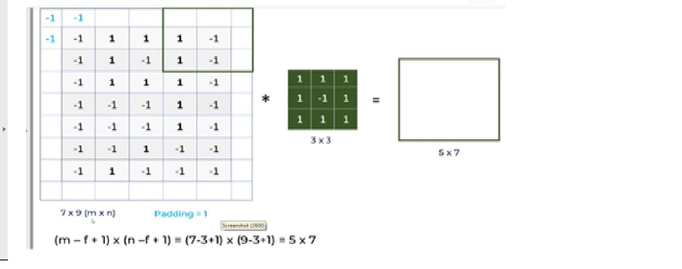
Let’s discuss what is problem with CNN and how the padding operation will solve the problem.
a. For a gray scale (n x n) image and (f x f) filter/kernel, the dimensions of the image resulting from a convolution operation is (n – f + 1) x (n – f + 1).
So for instances, a 5*7 image and 3*3 filter kernel size, the output result after convolution operation would be a size of 3*5. Thus, the image shrinks every time after the convolutional operation
b. Pixels, located on corners are contributed very little compared to middle pixels.
So, then to mitigate these problems, padding operation is done. Padding is a simple process of adding layers with 0 or -1 to input images so to avoid above mentioned problems.
Here we are using Padding = Same arguments, which depicts that output images have the same dimensions as input images.
· Activation Function – Relu
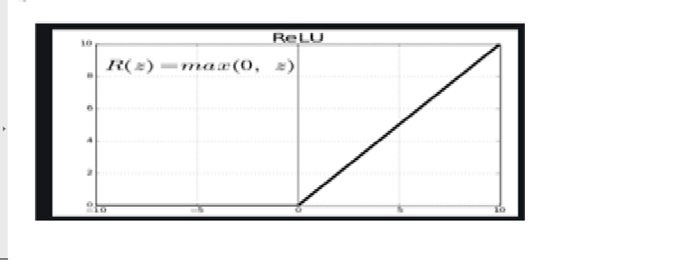
Since images are non-linear, to bring non-linearity, the relu activation function is applied after the convolutional operation.
Relu stands for Rectified linear activation function. Relu function will output the input directly if it is positive, otherwise, it will output zero.
· Input shape
This argument shows image size – 224*224*3. Since the images in RGB format so, the third dimension of the image is 3.
3. Pooling Operation
Python Code :
model.add(MaxPooling2D(pool_size=2))
We need to apply the pooling operation after initializing CNN. Pooling is an operation of down sampling of the image. The pooling layer is used to reduce the dimensions of the feature maps. Thus, the Pooling layer reduces the number of parameters to learn and reduces computation in the neural network.
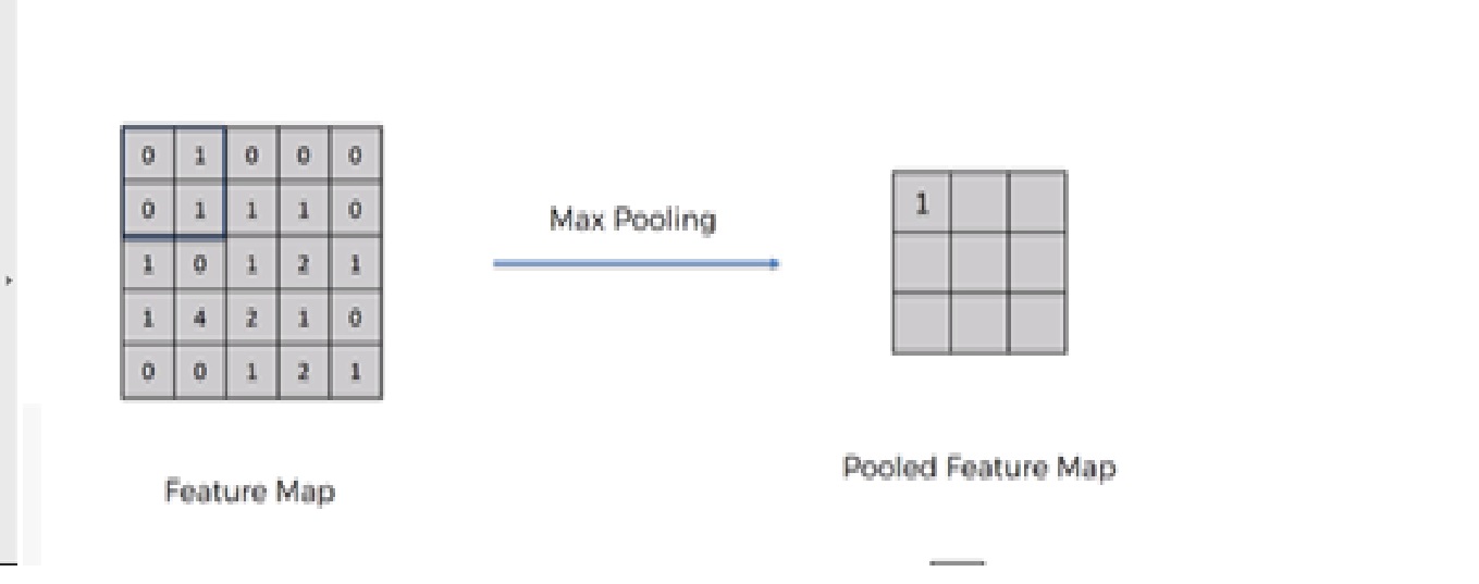
Future operations are performed on summarized features created by the pooling layer. instead of precisely positioned features generated by the convolution layer. This leads the model more robust to variations in the orientation of the feature in the image.
There are mainly 3 types of pooling: –
1. Max Pooling
2. Average Pooling
3. Global Pooling
4. Add two convolutional Layer
In order to add two more convolutional layers, we need to repeat steps 2 &3 with slight modification in the number of filters.
Python Code :
model.add(Conv2D(filters=32,kernel_size=2,padding="same",activation ="relu"))
model.add(MaxPooling2D(pool_size=2))
model.add(Conv2D(filters=64,kernel_size=2,padding="same",activation="relu"))
model.add(MaxPooling2D(pool_size=2))
We modified the 2nd and 3rd convolutional layers with filter numbers 32 & 64 respectively.
5. Flattening Operation
Python Code :
model.add(Flatten())
Flattening operation is converting the dataset into a 1-D array for input into the next layer which is the fully connected layer.
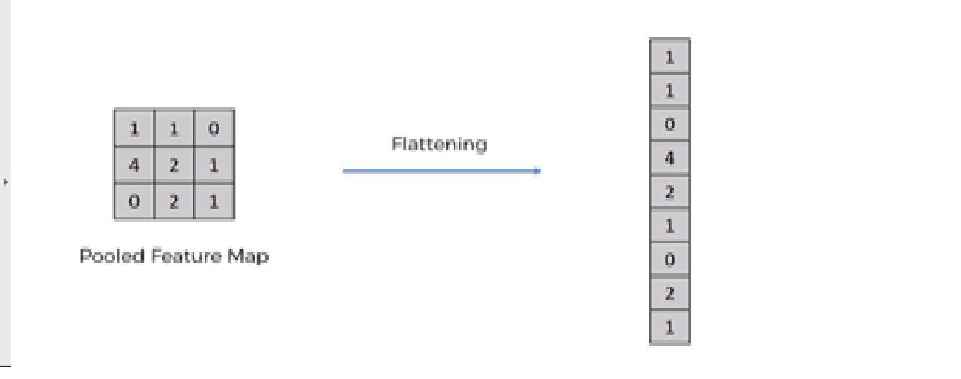
After finishing the 3 steps, now we have pooled feature map. We are now flattening our output after two steps into a column. Because we need to insert this 1-D data into an artificial neural network layer.
6. Fully Connected layer and output layer
The output of the flattening operation work as input for the neural network. The aim of the artificial neural network makes the convolutional neural network more advanced and capable enough of classifying images.
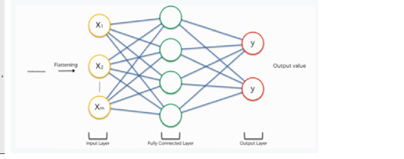
Here we are using a dense class from the Keras library from creating a fully connected layer and output layer.
Python Code :
model.add(Dense(500,activation="relu"))

model.add(Dense(2,activation="softmax"))
The softMax activation function is used for building the output layer. Let’s discuss the softmax activation function.
Softmax Activation Function
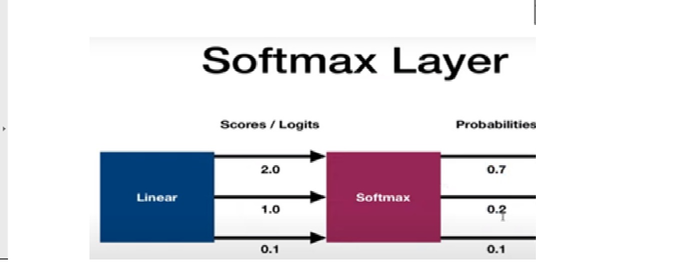
It is used as the last activation function of a neural network to bring the output of the neural network to a probability distribution over predicting classes. The output of Softmax is in probabilities of each possible outcome for predicting class. The probabilities sum should be one for all possible predicting classes.
Now, let’s discuss training and evaluation of the Convolutional neural network. We will be discussing this section in 3 steps;-
Step 1 – Compile CNN model
Step 2 – Fit model on training set
Step 3 – Evaluate Result
Step 1 – Compile CNN Model
Code line-
model.compile(loss=’categorical_crossentropy’,optimizer=’adam’,metrics=[‘accuracy’])
Here we are using 3 arguments:-
· Loss function
We are using the categorical_crossentropy loss function that is used in the classification task. This loss is a very good measure of how distinguishable two discrete probability distributions are from each other.
Kindly refer to the below link for a detailed discussion of different types of loss function:
· Optimizer
We are using adam Optimizer that is used to update neural network weights and learning rate. Optimizers are used to solve optimization problems by minimizing the function.
Kindly refer to the below link for a detailed explanation of different types of optimizer:
· Metrics arguments
Here, we are using Accuracy as a metrics to evaluate the performance of the Convolutional neural network algorithm.
Step 2 – Fit Model on Training Set
Code line:
model.fit_generator(training_set,validation_data=test_set,epochs=50, steps_per_epoch=len(training_set), validation_steps=len(test_set) )
We are fitting the CNN model on the training dataset with 50 iterations and each iteration has different steps for training and evaluating steps based on the length of the test and training set.
Step3:- Evaluate Result
We compare the accuracy and loss function for both the training and test dataset.
Code: Plotting loss graph
plt.plot(r.history['loss'], label='train loss')
plt.plot(r.history['val_loss'], label='val loss')
plt.legend()
plt.show()
plt.savefig('LossVal_loss')
Output
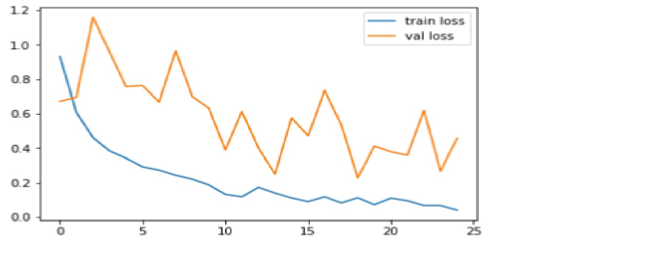
Loss is the penalty for a bad prediction. The aim is to make the validation loss as low as possible. Some overfitting is nearly always a good thing. All that matters, in the end, is: is the validation loss as low as you can get it.
Code: Plotting Accuracy graph
plt.plot(r.history['accuracy'], label='train acc')
plt.plot(r.history['val_accuracy'], label='val acc')
plt.legend()
plt.show()
plt.savefig('AccVal_acc')
Output
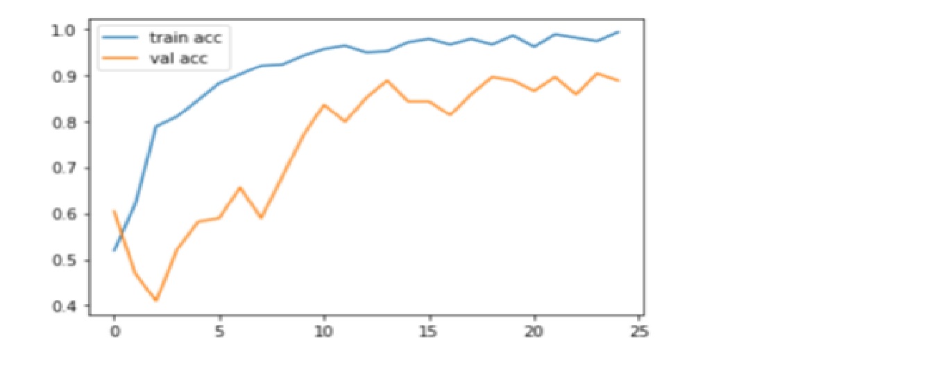
Accuracy is one metric for evaluating classification models. Informally, accuracy is the fraction of predictions our model got right. Here, we can observe that accuracy inches towards 90% on validating test which depicts a CNN model is performing well on accuracy metrics.
Thanks for reading! Happy Deep learning!!
References:
1. https://www.superdatascience.com/
2. https://www.youtube.com/watch?v=H-bcnHE6Mes
About Me :
I’m Jitendra Sharma, Data Science Intern at Nabler, pursuing PGDM-Big Data Analytics from Goa Institute of Management. You can contact me through LinkedIn and Github.
The media shown in this article are not owned by Analytics Vidhya and are used at the Author’s discretion.


