An Introduction to Logistic Regression

This article was published as a part of the Data Science Blogathon

Overview:

In this article, we will learn the in-depth working and implementation of Logistic Regression in Python using the Scikit-learn library.

Topics covered:

1. What is Logistic Regression?
2. Types of Logistic Regression
3. Extensions of Logistic Regression
4. Use Linear Regression for classification
5. How does Logistic Regression work?
6. Implementation in Python using Scikit-learn library

What is Logistic Regression?

Logistic Regression is a “Supervised machine learning” algorithm that can be used to model the probability of a certain class or event. It is used when the data is linearly separable and the outcome is binary or dichotomous in nature.

That means Logistic regression is usually used for Binary classification problems.

Binary Classification refers to predicting the output variable that is discrete in two classes.

A few examples of Binary classification are Yes/No, Pass/Fail, Win/Lose, Cancerous/Non-cancerous, etc.

Types of Logistic Regression

• Simple Logistic Regression: a single independent is used to predict the output
• Multiple logistic regression: multiple independent variables are used to predict the output

Extensions of Logistic Regression

Although it is said Logistic regression is used for Binary Classification, it can be extended to solve multiclass classification problems.

Multinomial Logistic Regression: The output variable is discrete in three or more classes with no natural ordering.

Food texture: Crunchy, Mushy, Crispy

Hair colour: Blonde, Brown, Brunette, Red​

Ordered Logistic Regression: Aka Ordinal regression model. The output variable is discrete in three or more classes with the ordering of the levels.

Customer Rating: extremely dislike, dislike, neutral, like, extremely like

Income level: low income, middle income, high income

Use Linear Regression for classification

Before moving ahead, spend some time to read my article on Simple Linear Regression in case you would want to brush up 🙂

Now, let us try if we can use linear regression to solve a binary class classification problem. Assume we have a dataset that is linearly separable and has the output that is discrete in two classes (0, 1).

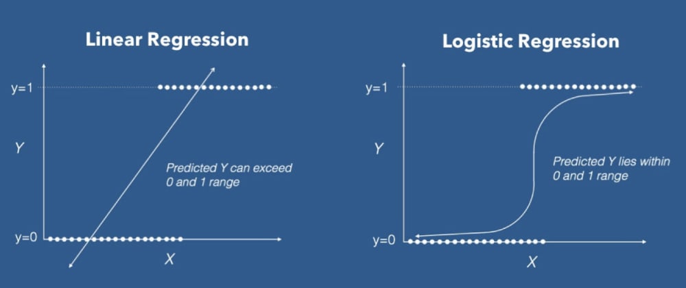
In Linear regression, we draw a straight line(the best fit line) L1 such that the sum of distances of all the data points to the line is minimal. The equation of the line L1 is y=mx+c, where m is the slope and c is the y-intercept.

We define a threshold T = 0.5, above which the output belongs to class 1 and class 0 otherwise.

Image by Author

Case 1: the predicted value for x1 is ≈0.2 which is less than the threshold, so x1 belongs to class 0.

Case 2: the predicted value for the point x2 is ≈0.6 which is greater than the threshold, so x2 belongs to class 1.

So far so good, yeah!

Case 3: the predicted value for the point x3 is beyond 1.

Case 4: the predicted value for the point x4 is below 0.

The predicted values for the points x3, x4 exceed the range (0,1) which doesn’t make sense because the probability values always lie between 0 and 1. And our output can have only two values either 0 or 1. Hence, this is a problem with the linear regression model.

Now, introduce an outlier and see what happens. The regression line gets deviated to keep the distance of all the data points to the line to be minimal.

L2 is the new best-fit line after the addition of an outlier. Seems good till now. But the problem is, if we closely observe, some of the data points are wrongly classified. Certainly, it increases the error term 🙁 This again is a problem with the linear regression model.

The two limitations of using a linear regression model for classification problems are:

• the predicted value may exceed the range (0,1)
• error rate increases if the data has outliers

There definitely is a need for Logistic regression here.

How does Logistic Regression Work?

The logistic regression equation is quite similar to the linear regression model.

Consider we have a model with one predictor “x” and one Bernoulli response variable “ŷ” and p is the probability of ŷ=1. The linear equation can be written as:

p = b0+b1x     --------> eq 1

The right-hand side of the equation (b₀+b₁x) is a linear equation and can hold values that exceed the range (0,1). But we know probability will always be in the range of (0,1).

To overcome that, we predict odds instead of probability.

Odds: The ratio of the probability of an event occurring to the probability of an event not occurring.

Odds = p/(1-p)

The equation 1 can be re-written as:

p/(1-p) = b0+b1x      --------> eq 2

Odds can only be a positive value, to tackle the negative numbers, we predict the logarithm of odds.

Log of odds = ln(p/(1-p))

The equation 2 can be re-written as:

ln(p/(1-p)) = b0+b1x      --------> eq 3

To recover p from equation 3, we apply exponential on both sides.

exp(ln(p/(1-p))) = exp(b0+b1x)
eln(p/(1-p)) = e(b0+b1x)

From the inverse rule of logarithms,

p/(1-p) = e(b0+b1x)

Simple algebraic manipulations

p = (1-p) * e(b0+b1x)
p = e(b0+b1x)- p * e(b0+b1x)

Taking p as common on the right-hand side

p = p * ((e(b0+b1x))/p - e(b0+b1x))
p = e(b0+b1x) / (1 + e(b0+b1x))

Dividing numerator and denominator by e^(b0+b1x) on the right-hand side

p = 1 / (1 + e-(b0+b1x))

Similarly, the equation for a logistic model with ‘n’ predictors is as below:

p = 1/ (1 + e-(b0+b1x1+b2x2+b3x3+----+bnxn)

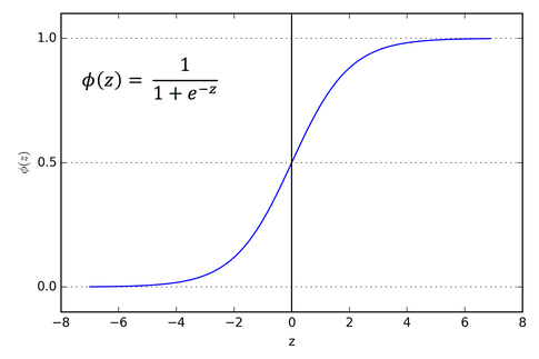
The right side part looks familiar, isn’t it? Yes, it is the sigmoid function. It helps to squeeze the output to be in the range between 0 and 1.

Sigmoid Function:

The sigmoid function is useful to map any predicted values of probabilities into another value between 0 and 1.

Source

We started with a linear equation and ended up with a logistic regression model with the help of a sigmoid function.

Linear model: ŷ = b₀+b₁x
Sigmoid function: σ(z) = 1/(1+e^−z)
Logistic regression model: ŷ = σ(b₀+b₁x) = 1/(1+e^-(b0+b1x))

So, unlike linear regression, we get an ‘S’ shaped curve in logistic regression.

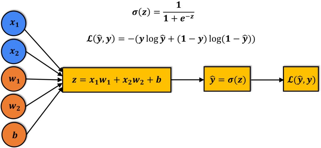
The image that depicts the working of the Logistic regression model

A linear equation (z) is given to a sigmoidal activation function (σ) to predict the output (ŷ).

To evaluate the performance of the model, we calculate the loss. The most commonly used loss function is the mean squared error.

But in logistic regression, as the output is a probability value between 0 or 1, mean squared error wouldn’t be the right choice. So, instead, we use the cross-entropy loss function.

The cross-entropy loss function is used to measure the performance of a classification model whose output is a probability value.

Learn more about the cross-entropy loss function from here.

Kudos to us, we have steadily come all the way here and understood the limitations of Linear regression for classification and the working of the Logistic regression model.

It’s time a take a small break ☕ and come back for the implementation part.

Implementation in Python using Scikit-learn library

For classification, I am using a popular Fish dataset from Kaggle. I’ve added the dataset to my GitHub repository for easy access.

Define the dataset URL

dataset_url = "https://raw.githubusercontent.com/harika-bonthu/02-linear-regression-fish/master/datasets_229906_491820_Fish.csv"

# Create a pandas data frame from the fish dataset

import pandas as pd
fish = pd.read_csv(dataset_url, error_bad_lines=False)
fish.head()

Checking unique categories of the target feature. Our dataset has information about 7 fish species

fish[‘Species’].unique()

Check if there are any null values. Our dataset has no null values.

fish.isnull().sum()

Defining input and target variables

X = fish.iloc[:, 1:]
y = fish.loc[:, 'Species']

Scaling the input features using MinMaxScaler

from sklearn.preprocessing import MinMaxScaler
scaler = MinMaxScaler()
scaler.fit(X)
X_scaled = scaler.transform(X)

Label Encoding the target variable using LabelEncoder

from sklearn.preprocessing import LabelEncoder
label_encoder = LabelEncoder()
y = label_encoder.fit_transform(y)

Splitting into train and test datasets using train_test_split

from sklearn.model_selection import train_test_split
X_train, X_test, y_train, y_test= train_test_split(X_scaled, y, test_size=0.2, random_state=42)

Model Building and training

from sklearn.linear_model import LogisticRegression
clf = LogisticRegression()
# training the model
clf.fit(X_train, y_train)

Predicting the output

y_pred = clf.predict(X_test)

Computing the accuracy

from sklearn.metrics import accuracy_score
accuracy = accuracy_score(y_test, y_pred)
print("Accuracy: {:.2f}%".format(accuracy * 100))

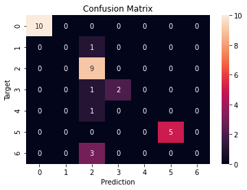
Our model achieved 81.25% accuracy, which is pretty good.

Confusion Matrix

from sklearn.metrics import confusion_matrix
cf = confusion_matrix(y_test, y_pred)
plt.figure()
sns.heatmap(cf, annot=True)
plt.xlabel('Prediction')
plt.ylabel('Target')
plt.title('Confusion Matrix')

References:

Logistic Regression Wikipedia

Kaggle Fish dataset URL

Scikit-learn LogisticRegression

End Notes:

 Thank you for reading till the conclusion. By the end of this article, we are familiar with the working and implementation of Logistic regression in Python using the Scikit-learn library.

I hope you enjoyed reading this article, feel free to share it with your study buddies 😊

Other Blog Posts by me

Feel free to check out my other blog posts from my Analytics Vidhya Profile.

You can find me on LinkedIn, Twitter in case you would want to connect. I would be glad to connect with you.

For immediate exchange of thoughts, please write to me at [email protected]

Harika

Hi, my name is Harika. I am a Data Engineer and I thrive on creating innovative solutions and improving user experiences. My passion lies in leveraging data to drive innovation and create meaningful impact.