This article was published as a part of the Data Science Blogathon
Introduction
What are Data Distributions in Probability and statistics?
Why we use Distributions in Probability and Statistics:
So the question is why we are using these distributions in probability and statistics. The intuition of using these distributions is very straightforward, we simply want to know the answer to various questions about the data or random variable. And here comes the two amazing fields of mathematics called probability and statistics. Probability and statistics have the strength to give the answers to our questions using some simple calculations.
Statistics and probability provide us the power to know about the data without even looking at the data. So probability and statistics provide us the various types of distributions such as Gaussian (aka Normal), Bernoulli, Binominal, Log-Normal, Perito distribution, etc. If we just know that the data or random variable follows any of the distribution available in probability and statistics we can answer tons of questions related to the data, that’s why we use distributions in probability and statistics.
Mean, Variance, Pdf, and CDF:
Before we start learning about the Empirical rule we need to understand the concept of Mean, variance, pdf, and CDF because without knowing these terms we cant imagine the distributions so let’s learn about these topics:
Mean: Mean is nothing but the average of all data points. We simply calculate the mean by dividing the sum of all data points by the number of all data points and it is denoted by μ. Mean it gives us the central tendency of data points.
The formula of Mean is as follows:

created in paint
Where xi is each dada point in random variable X, and n is the number of data points.
Variance: Variance is nothing but the average squared distance between each data point to the mean value. variance tells about the spread of our distribution. in other words the variance tells us how far the data point is spread from the mean value. the variance is denoted by the symbol σ2.
The formula of Variance is as follows:
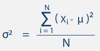
https://getcalc.com/formula/statistics/variance-population-data.png
and if we take the square root of the variance σ2 Then it’s become a Standard Deviation which is denoted by σ .
Pdf ( Probability Density Function ): Pdf is the smooth form of histograms which, pdf is defined as the density of data points on the particular value of the random variable. in other words, pdf is the measure of the density of data points in the given range of the data.
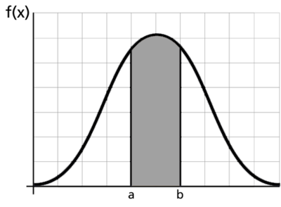
In the above figure, the density of points or the counts of the points between the range a and b. By looking at the figure we literally can say that there are more data points of random variable lies between the range of a and b.
CDF ( Cumulative Distribution Function ): The cumulative distribution function is the method to describe the random variable. This function shows us that how much % of data points lie in the range of 0 to a given point. Or in other words, it tells us what is the location of our given data point on the 100% distribution of data.
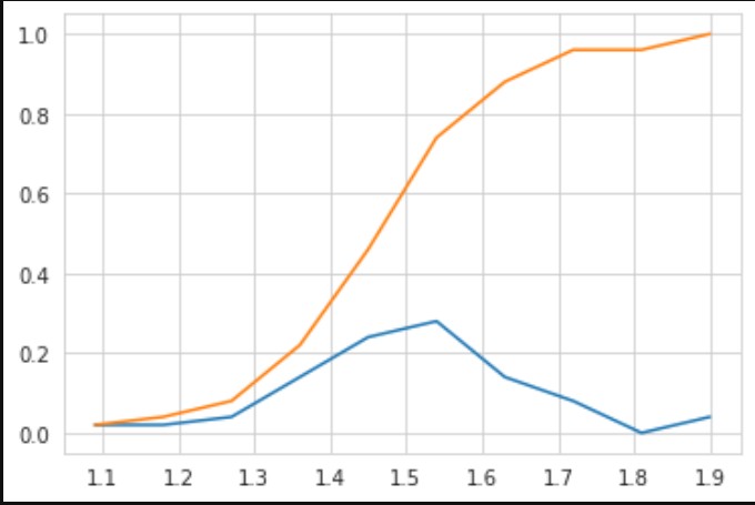
In the above figure, the blue line is called Pdf and the orange line is called CDF, the value of CDF is always lie between 0 to 1. if we draw the perpendicular on the x-axis then there is a point that exists on the graph somewhere cut the CDF function, and if we perpendicularly join the cross point of CDF to the y axis then you find the probability of data point of the x-axis on the y axis. for example, if your value of the x-axis is 1.5, then if you follow the above method of drawing perpendicular, then you will find that there are 60% of points exist in the distribution which value is less than or equal to 1.5.
68-95-99.7 % Rule or Empirical Rule:
We get to see this rule under the Normal or Gaussian distribution. whenever a data or random variable follows the normal distribution, then we can apply this rule to the data. So let’s get to know a little bit about the Gaussian distribution.
Gaussian distribution is symmetric distribution. This means if we draw the Probability Density Function ( Pdf ) of normal distribution then the Pdf of both sides of the mean value will be the mirror image of each other. The Pdf of the Gaussian distribution is a bell-shaped curve that is symmetric.
Let’s assume that X is a random variable and follows Gaussian distribution with some mean (μ) and Standard deviation (σ)

created in paint
So in the gaussian distribution, inside the bell curve the central point is our mean value, and if we just add standard deviation to the mean (μ + σ) and subtract standard deviation to the mean (μ – σ), then the range we get is called the range of first standard deviation. similarly, if we add 2 * standard deviation to the mean ( μ + 2σ) and subtract 2 * standard deviation to the mean (μ – 2σ) then we got the range of second standard deviation.
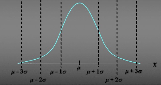
So according to the Empirical rule, if a random variable follows Gaussian distribution then it has also three properties, and these properties are also called the Empirical formula or 68-95-99.8 % formula, and the three properties of the Empirical formula are as follows:
1. P [ μ – σ <= X <= μ + σ ] ≈ 68 %
So the first formula basically says that the probability of a variable that falls within the range of μ – σ and μ + σ is 68 %. which means 68 % of the data points belonging to the random variable X fall within the range of the first standard deviation.
2. P [ μ – 2σ <= X <= μ + 2σ ] ≈ 95 %
So the second formula basically says that the probability of a variable that falls within the range of μ – 2σ and μ + 2σ is 95 %. which means 95% of the data points belonging to the random variable X fall within the range of the second standard deviation.
3. P [ μ – 3σ <= X <= μ + 3σ ] ≈ 99.8 %
So the second formula basically says that the probability of a variable that falls within the range of μ – 3σ and μ + 3σ is 99.8 %. which means 99.8% of the data points belonging to the random variable X fall within the range of the third standard deviation.
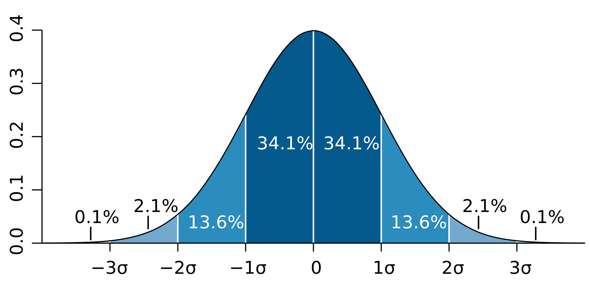
So I hope you understand the idea of Empirical rule,
Thank you.


