Complete guide on how to Use LightGBM in Python

Introduction

A Gradient Boosting Decision Tree (GBDT), such as LightGBM in Python, is a highly favored machine learning algorithm renowned for its effectiveness. Alongside implementations like XGBoost, it offers various optimization techniques. However, despite its popularity, the efficiency and scalability of the model can falter when handling datasets with numerous features. This limitation stems from the fact that each feature needs to scan through all data instances to estimate potential split points, a process that proves time-consuming and tedious.

To solve this problem, The LightGBM algorithm or Light Gradient Boosting Model is used. It uses two types of techniques which are gradient Based on side sampling or GOSS and Exclusive Feature bundling or EFB. So GOSS will actually exclude the significant portion of the data part which have small gradients and only use the remaining data to estimate the overall information gain. The data instances which have large gradients actually play a greater role for computation on information gain. GOSS can get accurate results with a significant information gain despite using a smaller dataset than other models.

With the EFB, It puts the mutually exclusive features along with nothing but it will rarely take any non-zero value at the same time to reduce the number of features. This impacts the overall result for an effective feature elimination without compromising the accuracy of the split point.

Learning Objectives:

• Understand the core principles and advantages of LightGBM continue training
• Learn to implement LightGBM in Python for classification tasks
• Interpret LightGBM’s feature importance and evaluation metrics
• Compare LightGBM’s performance with other gradient boosting algorithms

This article was published as a part of the Data Science Blogathon

What is LightGBM(Light gradient Boosting Machine)?

LightGBM is a powerful and efficient open-source gradient boosting framework for machine learning. It’s specifically designed to handle large datasets and perform well in terms of speed and memory usage. LightGBM continue training uses a technique called gradient boosting, which combines multiple weak learners (usually decision trees) to create a strong predictive model.

Demystifying the Maths behind LightGBM in Python

We use a concept known as verdict trees so that we can cram a function like for example, from the input space X, towards the gradient space G. A training set with the instances like x₁,x₂ and up to x_n is assumed where each element is a vector with s dimensions in the space X. In each of the restatements of a gradient boosting, all the negative gradients of a loss function with respect towards the output model are denoted as g₁, g₂, and up to g_n. The decision tree actually divides each and every node at the most revealing feature, it also gives rise to the largest evidence gain. In this type of model, the data improvement can be measured by the variance after segregating. It can be represented by the following formula :

“Y=Base_tree(X)-lr*Tree1(X)-lr*Tree2(X)-lr*Tree3(X)”

Consider a training dataset O at a specific node of a decision tree. The variance gain of the dividing measure j at point d for a node is defined as follows:

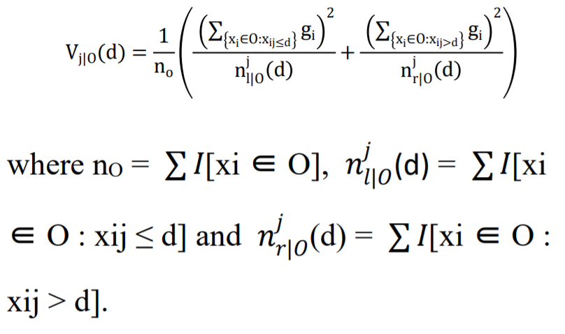
Gradient One-Sided Sampling or GOSS utilizes every instance with a larger gradient and does the task of random sampling on the various instances with the small gradients. The training dataset is represented by the symbol O for each specific node of the Decision tree. The variance gain of j, or the dividing measure at point d for the node, is expressed as:

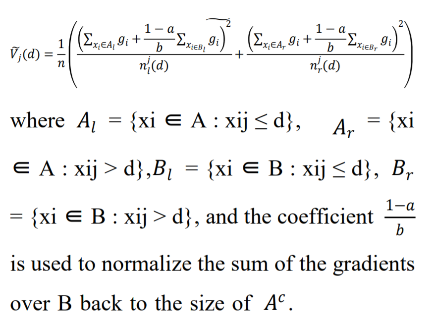
This is achieved by the method of GOSS in LightGBM models.

Coding an LGBM in Python

To install the LightGBM Python model, you can use the Python pip function by running the command “pip install lightgbm.” Moreover, LGBM features custom API support, enabling the implementation of both Classifier and regression algorithms. Both models operate similarly. The Titanic Passengers dataset will be used in the following code, and it is available in my drive at this location.

(Dataset Link: Click here)

Importing all the libraries

Python Code:

import lightgbm as lgb
import pandas as pd
import numpy as np
from sklearn.model_selection import train_test_split
from sklearn import metrics
#Loading the Data : 
data = pd.read_csv("SVMtrain.csv")
print(data.info())
print(data.head())
# train-test split---
x = data.drop(['Embarked','PassengerId'],axis=1)
y = data.Embarked
print("x dataset:---")
print(x.head())
print("y dataset:---")
print(y.head())

Output :

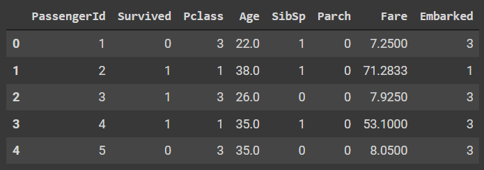
Here we can see that there are 8 columns out of which the passenger ID will be dropped and the embarked will be finally chosen as a target variable for the following classification challenge.

Loading the variables:

# To define the input and output feature
x = data.drop(['Embarked','PassengerId'],axis=1)
y = data.Embarked
# train and test split
x_train,x_test,y_train,y_test = train_test_split(x,y,test_size=0.33,random_state=42)

Loading and fitting the model:

The initial process of initializing a model is very similar to a normal model initializing and the main difference is that we will get much more parameter settings adjustments while we are initializing the model. We will define the max_depth, learning rate and random state in the following code. In the fit model, we have passed eval_matrix and eval_set to evaluate the model during training itself.

Code :

model = lgb.LGBMClassifier(learning_rate=0.09,max_depth=-5,random_state=42)
model.fit(x_train,y_train,eval_set=[(x_test,y_test),(x_train,y_train)],
          verbose=20,eval_metric='logloss')

Output:

Since our model has very low instances, we need to first check for overfitting with the following code and then we will proceed for the next few steps :

Code :

print('Training accuracy {:.4f}'.format(model.score(x_train,y_train)))
print('Testing accuracy {:.4f}'.format(model.score(x_test,y_test)))

Output :

Training accuracy 0.9647
Testing accuracy 0.8163

As we can clearly see that there is absolutely no significant difference between both the accuracies and hence the model has made an estimation that is quite accurate.

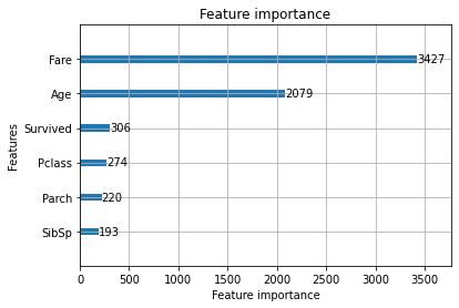
LGBM also comes with additional plotting functions like plotting the various feature importance, metric evaluation and the tree plot.

Code :

lgb.plot_importance(model)

Output :

If you do not mention the eval_set during the fitment, then you will actually get an error while plotting the metric evaluation

Code :

lgb.plot_metric(model)

Output

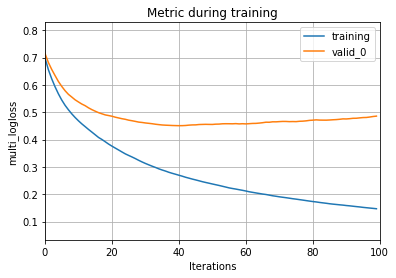
And as you can clearly see here, the validation curve will tend to increase after it has crossed the 100th evaluation. This can be totally fixed by tuning and setting the hyperparameters of the model. We can also plot the tree using a function.

Code:

lgb.plot_tree(model,figsize=(30,40))

Output:

Now we will plot a few metrics by using the sklearn library

Code :

metrics.plot_confusion_matrix(model,x_test,y_test,cmap='Blues_r')

Output :

Code :

print(metrics.classification_report(y_test,model.predict(x_test)))

Output :

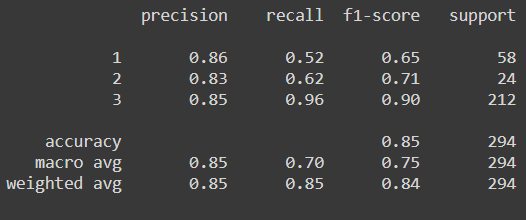
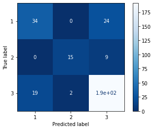
Now as we can clearly see from the confusion matrix combined with the classification report, the model is struggling to predict class 1 because of the few instances that we have but if we compare the same result with the other various ensemble algorithm, then LGBM performs the best. We can also perform the same process for the regressor model but there we need to change the estimator to the LGBMRegressor()

Conclusion

LightGBM proves to be a powerful tool in the machine learning landscape, offering significant advantages in speed, memory efficiency, and accuracy. Its innovative techniques like GOSS and EFB enable it to handle large datasets effectively while maintaining high performance. The practical implementation in LightGBM Python, as demonstrated, showcases LightGBM’s ease of use and interpretability through built-in visualization tools. While it excels in many scenarios, users should consider dataset characteristics and specific requirements when choosing between LightGBM continue training and other algorithms. Overall, LightGBM stands as a valuable asset for data scientists tackling complex predictive modeling tasks.

The media shown in this article are not owned by Analytics Vidhya and are used at the Author’s discretion.

Frequently Asked Questions

Arnab M

I love to code and create new software for any purpose. I also love to play MMO and RTG games. Other hobbies include Exploring new places and restaurants and making new friends. Feel free to ping me on LinkedIn for any new ideas or same and if you need any help with any code too.