This article was published as a part of the Data Science Blogathon
Introduction
When we start working on any Computer Vision-based task few issues that are faced by all of us are either lack of data or the quality of the data. Having less amount of data still has only two possible solutions, one is to try to get more data or go ahead with the different augmentation techniques, but when we talk about the quality of data that differs a lot since all the images that you have would not have been clicked under some restricted guidelines. A user can click images under different lighting conditions, various angles, and DPI so it is a kind of NP-hard problem to come with an ideal image enhancement technique that would work for all of them.
So there are a set of methods that are mainly used for enhancing image quality for computer vision tasks like object detection, image classification, OCR, etc. We would be discussing them one by one by taking an example image and applying all kinds of enhancing techniques.
Techniques that we are going to discuss in this article are as follows:
- Binarisation / Thresholding
- Noise Reduction
- Remove Skewness / Deskew
- Rescaling
- Morphological Operations
- for trying out these operations we would be using Python3 language and its two libraries Pillow and OpenCV.
Binarisation
This technique is used for converting an image from RGB to a Monochrome (Black and White) and is often referred to as Thresholding. This technique is mainly used for OCR tasks that require black text on white background.
OCR models are trained on images that have black text on white background in order to come up with better accuracy, so binarising an image helps in improving the quality of the OCR model. Binaraising an image also helps to save space and fasten the processing as it has only one color channel as compared to other multichannel image formats.
There are several types of Binarisation techniques provided by the OpenCV library.
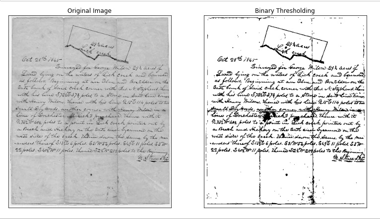
1. Binary Thresholding: This is the simplest one where we have to define a threshold and below that threshold, all the pixel values are converted to black and rest into white which results in a binarised image, you can use the following code snippet to apply binary thresholding to an image.
## import dependencies
import cv2
from PIL import Image
import matplotlib.pyplot as plt
## reading image
img = cv2.imread('text_document.jpg',0)
## apply binary thresholding
ret,thresh1 = cv2.threshold(img,170,255,cv2.THRESH_BINARY)
## plot original and binarised image
titles = ['Original Image', 'Binary Thresholding']
images = [img, thresh1]
for i in range(2):
    plt.figure(figsize=(20,20))
    plt.subplot(2,3,i+1),plt.imshow(images[i],'gray',vmin=0,vmax=255)
    plt.title(titles[i])
    plt.xticks([]),plt.yticks([])
The above code would result in the following image:
2. Adaptive Thresholding: Unlike binary thresholding, this method determines the threshold for a pixel value based on its small surrounding region. This method is also of two types:
- Adaptive Mean Thresholding: The threshold value is the mean of the neighborhood area minus the constant C.
- Adaptive Gaussian Thresholding: The threshold value is a gaussian-weighted sum of the neighborhood values minus the constant C.
This method is mainly used for removing different lighting conditions in an image since we get the pixel values based on their surrounding regions.
## import dependencies

import cv2

from PIL import Image

import matplotlib.pyplot as plt

## reading image

img = cv2.imread('lighting_conditions.jpg', 0)

## apply adaptive thresholding

## adaptive mean thresholding

th1 = cv2.adaptiveThreshold(img,255,cv2.ADAPTIVE_THRESH_MEAN_C,

            cv2.THRESH_BINARY,11,2)

## adaptive gaussian thresholding

th2 = cv2.adaptiveThreshold(img,255,cv2.ADAPTIVE_THRESH_GAUSSIAN_C,

            cv2.THRESH_BINARY,11,2)

## plot original and binarised image

titles = ['Original Image', 'Adaptive Mean Thresholding', 'Adaptive Gaussian Thresholding']

images = [img, th1, th2]

plt.figure(figsize=(20,20))

for i in range(3):

    plt.subplot(2,3,i+1),plt.imshow(images[i],'gray',vmin=0,vmax=255)

    plt.title(titles[i])

    plt.xticks([]),plt.yticks([])
The output of the above code is as follows:

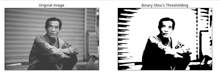
3. Otsu’s Binrisation: This method does not require any thresholding parameter as it automatically determines it. This method determines the threshold value by creating a histogram of all the pixel values and then calculating the mean value out of it.
## import dependencies

import cv2

from PIL import Image

import matplotlib.pyplot as plt

## reading image

img = cv2.imread('lighting_conditions.jpg', 0)

## apply Otru's thresholding

ret3,th1 = cv2.threshold(img,0,255,cv2.THRESH_BINARY+cv2.THRESH_OTSU)

## plot original and binarised image

titles = ["Original Image", "Binary Otsu's Thresholding"]

images = [img, th1]

plt.figure(figsize=(20,20))

for i in range(2):

    plt.subplot(2,3,i+1),plt.imshow(images[i],'gray',vmin=0,vmax=255)

    plt.title(titles[i])

    plt.xticks([]),plt.yticks([])
The output of the above code is as follows:
Noise Reduction
The most important factor because of which most of the computer vision tasks fail is Noise. Noise can be a Gaussian Noise (arose due to different lighting conditions) and Salt and Paper Noise (sparse light and dark disturbances).
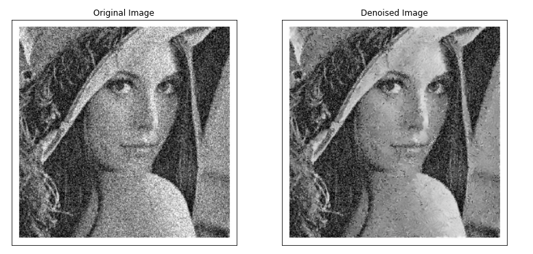
Sometimes images look nicer to human eyes but when we pass those images to any Computer Vision-based model like classification and object detection results do not come up well as due to noise object which we want to find is distorted and may not match with the one on which the model was trained, so noise in an image can degrade your model’s accuracy.
OpenCV provides a function called fastNIMeansDenoising() that smoothens the images in order to reduce the image noise.
## import dependencies

import cv2

from PIL import Image

import matplotlib.pyplot as plt

## reading image

img = cv2.imread('noisy_image.jpg')

## apply image denoising

dst = cv2.fastNlMeansDenoisingColored(img,None,10,10,7,21)

## plot original and denoised image

titles = ["Original Image", "Denoised Image"]

images = [img, dst]

plt.figure(figsize=(20,20))

for i in range(2):

    plt.subplot(2,3,i+1),plt.imshow(images[i],'gray',vmin=0,vmax=255)

    plt.title(titles[i])

    plt.xticks([]),plt.yticks([])
The above code would result in the following image:
Deskew
Deskew is the process of removing the skewness (angle different than 0) from the image. There are no concrete solutions for this issue. You might find multiple solutions for this on the web but when you would be trying out those on your images it might not make sense to you. So I would suggest you train your own Computer Vision-based model, creating a classification model that classifies multiple angle images is the best choice.
Rescaling
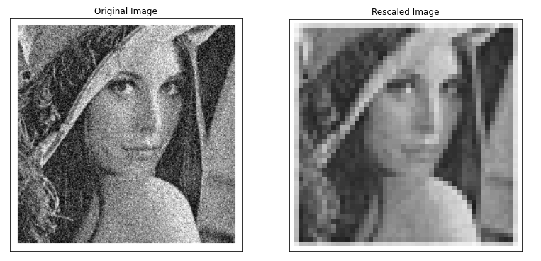
Rescaling is the process of enlarging or shrinking down your image so that the resolution of the image is changed. When you rescale an image, different pixel values in that image are replicated to make it more pixelated and pixel values are removed in order to get it downscaled. This method is mainly used in Image Classification and Object Detection, as there you need to rescale the image to the model input size.
Suppose you are creating a VGG classifier for types of cat and dog classes, there you have some images which might not be of the same size, so you can not pass those images as they are to the model as the model expects a fixed image size. In that case, you need to either scale down or scale up the image size based on the model’s input size.
A simple way to rescale your image is as follows:
## import dependencies
import cv2
from PIL import Image
import numpy as np
import matplotlib.pyplot as plt
## reading image
img = Image.open('noisy_image.jpg')
## apply image rescaling and making image 300x300 (downscaling)
dst = img.resize((50,50))
## plot original and downscaled image
titles = ["Original Image", "Rescaled Image"]
images = [np.asarray(img), np.asarray(dst)]
plt.figure(figsize=(20,20))
for i in range(2):
    plt.subplot(2,3,i+1),plt.imshow(images[i],'gray',vmin=0,vmax=255)
    plt.title(titles[i])
    plt.xticks([]),plt.yticks([])
The above code would result in the following image:
Morphological Operations
Morphological operations are some simple forms of operations that are used for image transformation. For image transformation, the input image array is multiplied with a kernel which decides the nature of the operation.
When you have some object whose boundary you are not able to see clearly you can use the morphological operation to widen its boundary and that would help to find the objects easily, similarly, if the boundary is large you can shrink it down with the same. These techniques are mainly used for ICR as their text boundaries are smaller and need to be magnified in order for ICR models to recognize them.
Two main types of morphological operations are as follows:
1. Erosion: This operation tries to erode the foreground of the image and resulting in minimizing the white pixel values from the image. The extent of erosion is totally dependent on the size of the kernel and the number of iteration you apply that kernel for. The kernel is a square-size matrix having only ones and zeros values to come up with the eroded images.
Erosion using 5×5 matrix applied for one iteration looks like the following:
## import dependencies
import cv2
from PIL import Image
import matplotlib.pyplot as plt
## reading image
img = cv2.imread('text_document.jpg', 0)
## apply erosion
kernel = np.ones((5,5),np.uint8)
erosion = cv2.erode(img,kernel,iterations = 1)
## plot original and eroded image
titles = ["Original Image", "Eroded Image"]
images = [img, erosion]
plt.figure(figsize=(20,20))
for i in range(2):
    plt.subplot(2,3,i+1),plt.imshow(images[i],'gray',vmin=0,vmax=255)
    plt.title(titles[i])
    plt.xticks([]),plt.yticks([])
The resultant image is as follows:
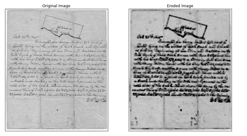
Image 6
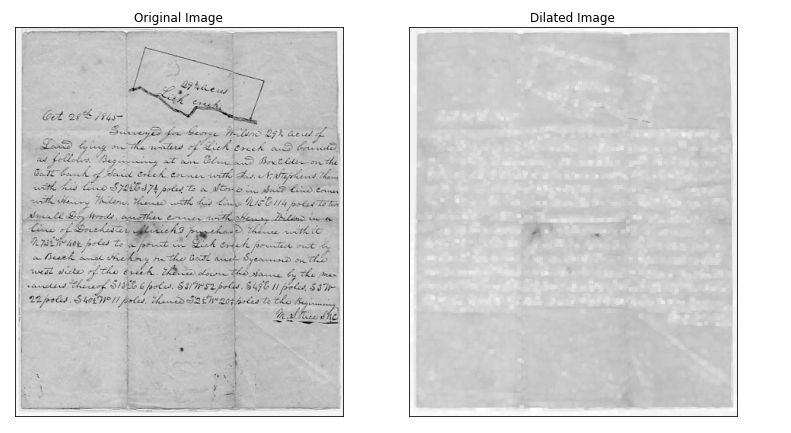
2. Dilation: This operation is the opposite of erosion which tries to maximize the white areas in images. This is also dependent on the kernel size and number of iterations.
Dilations using 5×5 kernel size for 1 iteration looks like following:
## import dependencies
import cv2
from PIL import Image
import matplotlib.pyplot as plt
## reading image
img = cv2.imread('text_document.jpg', 0)
## apply dilation
kernel = np.ones((5,5),np.uint8)
dilation = cv2.dilate(img,kernel,iterations = 1)
## plot original and dilated image
titles = ["Original Image", "Dilated Image"]
images = [img, dilation]
plt.figure(figsize=(20,20))
for i in range(2):
    plt.subplot(2,3,i+1),plt.imshow(images[i],'gray',vmin=0,vmax=255)
    plt.title(titles[i])
    plt.xticks([]),plt.yticks([])
Conclusion
So these are some of the most important techniques which you can use to improve the quality of the images and hence resulting in increased accuracy of the Computer Vision-based model. There is no proper way of selecting the algorithm it is totally based on trying out whatever works best for your data.
Sometimes the selection can be a solo and other times you would have to use a combination of these algorithms in order to make your data more suitable for your algorithm. In conclusion, if the quality of your images is too bad and you want these algorithms to work on those images there you would have some dissatisfaction as these techniques can improve images having less noise and impurities but for very bad images, it may not work.
Now you can go ahead and try out these operations based on your use case.
Thanks for reading this article do like if you have learned something new, feel free to comment See you next time !!! ❤️
Image Source-
- Image 1: surveyhistory.org
- Image 2 – digital-photography-school.com
- Image 3 – digital-photography-school.com
- Image 4 – researchgate.net
- Image 5 – researchgate.net
- Image 6 – surveyhistory.org
- Image 7 – surveyhistory.org


Nice article. Thank you for writing.
see you next time !!!