Introduction
Natural Language Processing has many applications these days. An important application of Natural Language Processing is text classification and text analytics. For this purpose, we need to create a classifier. But, the problem that lies in dealing with text data is that computers cannot directly understand natural language. Computers cannot simply take text input and understand the context of the text.
So, we use text vectorization for these cases. Term Frequency Inverse Document Frequency (TFIDF) analysis is one of the simple and robust methods to understand the context of a text. Term Frequency and Inverse Document Frequency is used to find the related content and important words and phrases in a larger text. Implementing TF-IDF analysis is very easy using Python. Computers cannot understand the meaning of a text, but they can understand numbers. The words can be converted to numbers so that the relationship between them can be understood.
This article was published as a part of the Data Science Blogathon
Table of contents
Term Frequency
The term is frequency measure of a word w in a document (text) d. It is equal to the number of instances of word w in document d divided by the total number of words in document d. Term frequency serves as a metric to determine a word’s occurrence in a document as compared to the total number of words in a document. The denominator is always the same.

Inverse Document Frequency (IDF)
This parameter gives a numeric value of the importance of a word. Inverse Document frequency of word w is defined as the total number of documents (N) in a text corpus D, divided by the number of documents containing w.

Term Frequency Inverse Document Frequency (TF-IDF)
The product of TF and IDF is the TF-IDF. TF-IDF is usually one of the best metrics to determine if a term is significant to a text. It represents the importance of a word in a particular document.
The issue with such methods is that they cannot understand synonyms, semantics, and other emotional aspects of language. For example, large and big are synonymous, but such methods cannot identify that.
Let us have a look at how to implement TF-IDF.
text=["kolkata big city india trade","mumbai financial capital india","delhi capital india","kolkata capital colonial times",
     "bangalore tech hub india software","mumbai hub trade commerce stock exchange","kolkata victoria memorial","delhi india gate",
      "mumbai gate way india trade business","delhi red fort india","kolkata metro oldest india",
      "delhi metro largest metro network india"]
Let us take some random text. A point to be noted is that text is not found like this usually. A lot of pre-processing has to be done to make the text like this. Next, we import the necessary libraries.
import pandas as pd
import numpy as np
from sklearn.feature_extraction.text import CountVectorizer
from sklearn.feature_extraction.text import TfidfTransformer
from sklearn.feature_extraction.text import TfidfVectorizer
The important libraries are thus imported.
Now, we apply count vectorizer to the text.
Python Code:
text=["kolkata big city india trade","mumbai financial capital india","delhi capital india","kolkata capital colonial times",
     "bangalore tech hub india software","mumbai hub trade commerce stock exchange","kolkata victoria memorial","delhi india gate",
      "mumbai gate way india trade business","delhi red fort india","kolkata metro oldest india",
      "delhi metro largest metro network india"]
import pandas as pd
import numpy as np
from sklearn.feature_extraction.text import CountVectorizer
from sklearn.feature_extraction.text import TfidfTransformer
from sklearn.feature_extraction.text import TfidfVectorizer
#using the count vectorizer
count = CountVectorizer()
word_count=count.fit_transform(text)
print(word_count)
Let us have a look at its shape.
word_count.shape
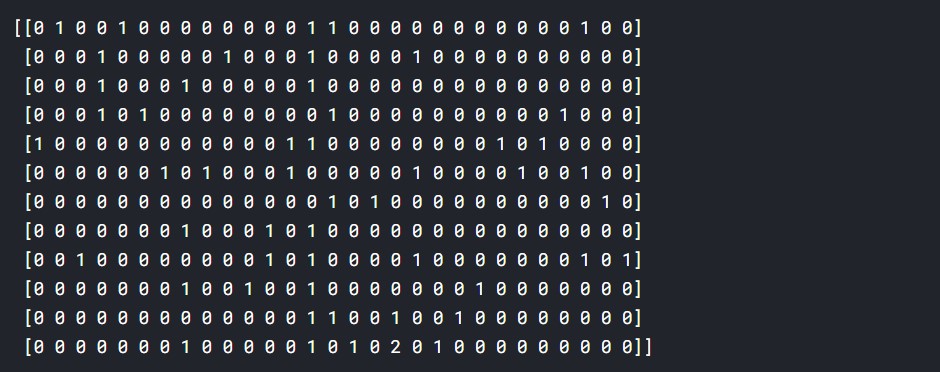
Let us now convert it into an array and have a look.
print(word_count.toarray())
We had taken 12 sentences, and there are 29 unique words, so the shape is 12/29.
Now, we use the IDF transformer.
tfidf_transformer=TfidfTransformer(smooth_idf=True,use_idf=True)
tfidf_transformer.fit(word_count)
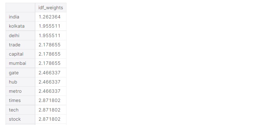
df_idf = pd.DataFrame(tfidf_transformer.idf_, index=count.get_feature_names(),columns=["idf_weights"])

#inverse document frequency
df_idf.sort_values(by=['idf_weights'])
Output is long, looks something like this. I will leave a link to the notebook, please have a look there.

Proceeding to the TF-IDF transformation.
#tfidf
tf_idf_vector=tfidf_transformer.transform(word_count)
feature_names = count.get_feature_names()

first_document_vector=tf_idf_vector[1]
df_tfifd= pd.DataFrame(first_document_vector.T.todense(), index=feature_names, columns=["tfidf"])

df_tfifd.sort_values(by=["tfidf"],ascending=False)
So, we can see that implementation of Term Frequency- Inverse Document Frequency is very simple and easy in Python.
Code link: https://www.kaggle.com/prateekmaj21/tf-idf-in-python
Creating a Movie Reviews Classifier using TF-IDF
Now, let us create a classifier to classify review texts as either positive or negative.
Necessary libraries are imported.
#importing libraries
import numpy as np
import pandas as pd
from sklearn.feature_extraction.text import TfidfVectorizer
from sklearn.naive_bayes import MultinomialNB
from sklearn import metrics
import nltk
import re
import string
from nltk.stem import WordNetLemmatizer
Now, reading the data.
#reading the data
test_csv = pd.read_csv('/kaggle/input/imdb-movie-reviews-dataset/test_data (1).csv')
train_csv = pd.read_csv('/kaggle/input/imdb-movie-reviews-dataset/train_data (1).csv')
After reading the data, we proceed with various text pre processing methods.
#stopword removal and lemmatization
stopwords = nltk.corpus.stopwords.words('english')
lemmatizer = WordNetLemmatizer()

nltk.download('stopwords')

train_csv.head()
We can see how the data consists of text, followed by a label of “1” or “0”. 1 indicates a positive review, whereas 0 indicates a negative review. Speaking of the data, text data is very complex to work with. There are punctuations, numbers and other special characters. Then, words of different cases are perceived differently. Stopwords also have to be removed. Words have to be lemmatized.
Stopwords are the most common words in a language, usually prepositions and articles. They are used a lot, but rather than conveying any sentiment or meaning, they are used for grammar. Stopwords are usually removed for an efficient NLP process.
Similarly, lemmatization is used to convert various forms of a word to the root format. Both are very important steps in the whole NLP process.
Now, we divide the data into training and testing parts.
train_X_non = train_csv['0']   # '0' refers to the review text
train_y = train_csv['1']   # '1' corresponds to Label (1 - positive and 0 - negative)
test_X_non = test_csv['0']
test_y = test_csv['1']
train_X=[]
test_X=[]
After this, we will do the important part of cleaning the text.
#text pre processing
for i in range(0, len(train_X_non)):
    review = re.sub('[^a-zA-Z]', ' ', train_X_non[i])
    review = review.lower()
    review = review.split()
    review = [lemmatizer.lemmatize(word) for word in review if not word in set(stopwords)]
    review = ' '.join(review)
    train_X.append(review)

#text pre processing
for i in range(0, len(test_X_non)):
    review = re.sub('[^a-zA-Z]', ' ', test_X_non[i])
    review = review.lower()
    review = review.split()
    review = [lemmatizer.lemmatize(word) for word in review if not word in set(stopwords)]
    review = ' '.join(review)
    test_X.append(review)
So, all the text processing is done properly.
Let us have a look at how the text data looks like now.
train_X[10]
We can see that punctuations are removed and all stopwords are also removed. This text can now be used to train a classifier.
Now, we use the TF-IDF Vectorizer.
#tf idf
tf_idf = TfidfVectorizer()
#applying tf idf to training data
X_train_tf = tf_idf.fit_transform(train_X)
#applying tf idf to training data
X_train_tf = tf_idf.transform(train_X)
Let us check the dimensions of the data now.
print("n_samples: %d, n_features: %d" % X_train_tf.shape)Output:

So, we can see that, there are 25,000 data points and 65498 features.
Now, we transform the test data into TF-IDF matrix format.
#transforming test data into tf-idf matrix
X_test_tf = tf_idf.transform(test_X)

print("n_samples: %d, n_features: %d" % X_test_tf.shape)
Output:

So, we can see that the number of features is the same. Now we can proceed with creating the classifier.
Naive Bayes Classifier
We shall be creating a Multinomial Naive Bayes model. This algorithm is based on Bayes Theorem. Multinomial Naive Bayes has many industries and commercial applications in the field of Natural Language Processing.
#naive bayes classifier
naive_bayes_classifier = MultinomialNB()
naive_bayes_classifier.fit(X_train_tf, train_y)

#predicted y
y_pred = naive_bayes_classifier.predict(X_test_tf)
Prediction is complete. Now, we print the classification report.
print(metrics.classification_report(test_y, y_pred, target_names=['Positive', 'Negative']))
Now, let us check the confusion matrix.
print("Confusion matrix:")
print(metrics.confusion_matrix(test_y, y_pred))
So, we can say that the classifier is performing pretty well.
Now, let us try a sample test prediction.
Doing a Test Prediction on Reviews Classifier Using TF-IDF
I have taken a sample positive review of the movie “Avatar”.
#doing a test prediction
test = ["This is unlike any kind of adventure movie my eyes have ever seen in such a long time, the characters, the musical score for every scene, the story, the beauty of the landscapes of Pandora, the rich variety and uniqueness of the flora and fauna of Pandora, the ways and cultures and language of the natives of Pandora, everything about this movie I am beyond impressed and truly captivated by. Sam Worthington is by far my favorite actor in this movie along with his character Jake Sulley, just as he was a very inspiring actor in The Shack Sam Worthington once again makes an unbelievable mark in one of the greatest and most captivating movies you'll ever see. "]
Next up is text pre-processing.
review = re.sub('[^a-zA-Z]', ' ', test[0])
review = review.lower()
review = review.split()
review = [lemmatizer.lemmatize(word) for word in review if not word in set(stopwords)]
test_processed =[ ' '.join(review)]
Let us have a look at the processed text.
test_processedOutput:
['unlike kind adventure movie eye ever seen long time character musical score every scene story beauty landscape pandora rich variety uniqueness flora fauna pandora way culture language native pandora everything movie beyond impressed truly captivated sam worthington far favorite actor movie along character jake sulley inspiring actor shack sam worthington make unbelievable mark one greatest captivating movie ever see']

test_input = tf_idf.transform(test_processed)
test_input.shape
Output:

It also has 65498 features.
#0= bad review
#1= good review
res=naive_bayes_classifier.predict(test_input)[0]
if res==1:
    print("Good Review")
elif res==0:
    print("Bad Review")
Output:

So, we can see that it is a Positive Review.
We successfully created a classifier.
Have a look at the code here: Github
Natural Language Processing has many widespread applications and text analytics and text classification is one of them. Hope this article explained creating a classifier using Python.
Conclusion
In conclusion, Natural Language Processing (NLP) plays a pivotal role in text classification and analytics. While computers struggle to understand natural language directly, techniques like Term Frequency Inverse Document Frequency (TF-IDF) provide a robust solution. This article showcased the implementation of TF-IDF using Python, illustrating its simplicity and effectiveness in converting text data into a numerical format understandable by computers. Furthermore, the creation of a movie reviews classifier demonstrated the practical application of TF-IDF in sentiment analysis. NLP continues to evolve, and mastering such techniques opens doors to diverse applications in data science. Explore the provided code on GitHub for hands-on learning.
Frequently Asked Questions
A. To use TF-IDF for classification in Python, employ libraries like scikit-learn. Preprocess text data, apply TF-IDF vectorization, and use a classification algorithm, such as Naive Bayes or SVM.
A. Classifying documents in TF-IDF involves transforming text into numerical features using TF-IDF vectorization. Then, apply a classification algorithm like Naive Bayes or SVM to predict document categories.
A. Obtain TF-IDF scores in Python using libraries like scikit-learn. Initialize a TF-IDF vectorizer, fit it to your text data, and transform the documents to get the TF-IDF matrix with corresponding scores.
A. The best algorithm for text classification depends on the dataset and requirements. Commonly used ones include Naive Bayes, SVM, and deep learning models like LSTM or BERT, with their effectiveness varying based on the task and data complexity.
The media shown in this article are not owned by Analytics Vidhya and are used at the Author’s discretion.


