This article was published as a part of the Data Science Blogathon
Introduction
Keras is a Python library that provides an API for dealing with Neural networks and Deep Learning frameworks. Keras provides methods and components that are useful while working with various Deep Learning applications in Python.
What is Keras for Deep Learning?
Previously, the most commonly used Deep Learning library was Tensorflow 1.x, which was challenging for beginners to work with. It took a lot of code to create a simple one-layer network. However, with Keras, the entire procedure of creating the structure of a Neural Network, as well as training and tracking it, became incredibly simple.
Keras is a high-level API that may be used with the Tensorflow, Theano, and CNTK backends. It enables us to perform neural network tests using a high-level and user-friendly API. It also has the ability to operate on CPUs and GPUs.

Keras APIs
Keras includes ten distinct API modules for modeling and training neural networks. Let’s go through some of them one by one.
Models
The Models API allows you to create complex neural networks by adding and deleting layers. The model might be Sequential, which means that the layers are packed sequentially with a single input and output. The model can also be functional, which means that it can be totally modifiable.
The API also includes a training module, which includes methods for compiling the model, as well as the optimizer and loss function, fitting the model, and evaluating and forecasting new data. It also includes methods for training, testing, and forecasting on batch data as well. Models API also supports model saving and serialization.
Types of Keras Models
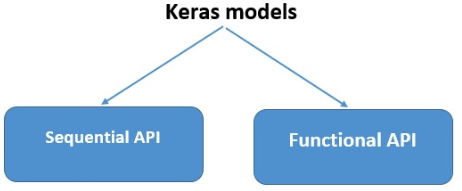
Keras models are classified into two types:
- Keras Sequential Model
- Keras Functional API

1. Sequential API in Keras
It enables us to build models layer by layer in sequential order. But it does not enable us to build models that have multiple inputs or outputs. It works well for basic stacks of layers with one input tensor and one output tensor.
When any of the layers in the stack contains multiple inputs or outputs, this model is ineffective. It is not suitable even if we want non-linear topology.
Here’s an example of a Sequential model:
from keras.models import Sequential
from keras.layers import Dense
model=Sequential()
model.add(Dense(64,input_shape=8,))
mode.add(Dense(32))
2. Functional API in Keras
It gives you greater flexibility when defining a model and adding layers in Keras. We can use the Functional API to construct models with multiple inputs and outputs. It also enables us to share these layers. In other words, we can create layer graphs using Keras’ functional API.
As we know a functional API is a data structure, it is easy to store it as a single file that can be used to recreate the exact model without having the original code. It’s also simple to model the graph and access its nodes from here.
The following is an example of a functional API:
from keras.models import Model
from keras.layers import Input, Dense
input=Input(shape=(32,))
layer=Dense(32)(input)
model=Model(inputs=input,outputs=layer)
//To create model with multiple inputs and outputs:
model=Model(inputs=[input1,input2],outputs=[layer1,layer2,layer3])
Layers in Deep Learning
Layers are the foundation of each and every neural network. The Layers API provides a comprehensive set of techniques for constructing the neural net architecture. The Base Layer class in the Layers API includes methods for creating custom layers with custom weights and initializers.
A Layer instance can be called in the same way as a function can:
from tensorflow.keras import layers
layer = layers.Dense(32, activation='relu')
inputs = tf.random.uniform(shape=(10, 20))
outputs = layer(inputs)
Layers, unlike functions, maintain a state that is updated as the layer gets input during training and saved in the layer. weights:
>>> layer.weights
[,
 ]
It includes the Layer Activations class, which has different activation functions such as ReLU, Sigmoid, Tanh, Softmax, and so on. The Layer Weight Initializers class provides methods for initializing weights in various ways.
It also includes the Core Layers class, which contains the classes needed to create core layers such as the Dense layer, Activation layer, Embedding layer, and so on. The Convolution Layer class provides several ways for adding various types of Convolution layers. The Pooling Layers class includes the methods needed for several forms of pooling, including Max Pooling, Average Pooling, Global Max Pooling, and Global Average Pooling.
Callbacks in Deep Learning
Callbacks are a method of tracking the model’s training process. With Callback enabled, you may conduct a variety of operations before or after the ending of an epoch or a batch.
You can use callbacks too:
- Saving the model to disc on a regular basis.
- Stopping early if the loss does not decrease significantly after a certain number of epochs.
- View a model’s internal states and statistics while it is being trained.
Dataset Preprocessing
The data is typically in raw format and organized in directories, and it must be preprocessed before being fed to the model for fitting. Many of these specialized functions may be found in the Image Data Preprocessing class. For example, the picture data must be in a numerical array, which may be accomplished with the img to array function. Alternatively, if the pictures are in a directory and subfolders, we may use the image_dataset_from_directory function.
The Data Preprocessing API also includes classes for Time Series data and text data.
Optimizers in Deep Learning
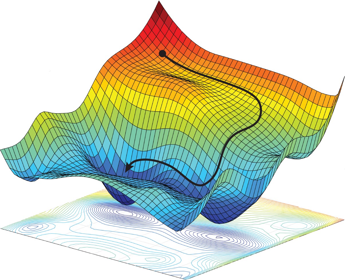
Optimizers are the core of any neural network. Every neural network optimizes a loss function in order to find the best weights for prediction. There are various types of optimizers, each of which uses somewhat different approaches to determine optimal weights. Optimizers such as SGD, RMSProp, Adam, Adadelta, Adagrad, Adamax, Nadal, and FTRL are all accessible via the Optimizers API.

Optimizers help Neural Networks in converting at the lowest position on the error surface, known as the minima. (Source)
Losses
When compiling a model, loss functions are must needed. The optimizer, which was also given as a parameter in the compilation procedure, would optimize this loss function. There are three types of losses: probabilistic losses, regression losses, and hinge losses.
Metrics
Every Machine Learning model uses metrics to quantify its performance on test data. Metrics are equivalent to Loss Functions, except they are performed on test data. Accuracy metrics include various types such as Accuracy, Binary Accuracy, Categorical Accuracy, and others. It also includes probabilistic metrics like binary cross-entropy, categorical cross-entropy, and so on. There are metrics for detecting false positives and negatives, such as AUC, Precision, Recall, and so on.
In addition to these classification metrics, it includes regression metrics such as Mean Squared Error, Root Mean Squared Error, Mean Absolute Error, and so on.
Keras Applications
The Keras Applications class includes several prebuilt models as well as pre-trained weights. These pre-trained models are utilized in the Transfer Learning process. These pre-trained models differ based on architecture, number of layers, trainable weights, etc. Some of them are VGG16, Xception, Resnet50, MobileNet, etc.
Using Keras for Neural Network Training
Consider a basic dataset like MNIST, which is accessible in Keras’ datasets class. We will create a simple sequential Convolutional Neural Network for categorizing the handwritten images of digits 0-9.
#Loading the dataset
 from keras.datasets import mnist
 (x_train, y_train), (x_test, y_test) = mnist.load_data()
By dividing each pixel by 255, the dataset is normalized. It’s also necessary to convert the pictures into four dimensions before feeding them to a CNN model.
x_train = x_train.astype(‘float32’)
 x_test = x_test.astype(‘float32’)
 x_train /= 255
 x_test /= 255
 x_train = X_train.reshape(X_train.shape[0], 28, 28, 1)
 x_test = X_test.reshape(X_test.shape[0], 28, 28, 1)
Before feeding the data to the model, we must label encode the classes. We’ll use Keras’ Utils class to do this.
from keras.utils import to_categorical
y_train = to_categorical(y_train, 10)
y_test = to_categorical(y_test, 10)
We can now begin building the model with Sequential API.
from keras.models import Sequential
 from keras.layers import Conv2D, MaxPool2D, Dense, Flatten, Dropoutmodel = Sequential()model.add(Conv2D(filters=32, kernel_size=(5,5), activation=‘relu’,  input_shape=x_train.shape[1:]))
 model.add(MaxPool2D(pool_size=(2, 2)))
 model.add(Dropout(rate=0.25))
 model.add(Conv2D(filters=64, kernel_size=(3, 3), activation=‘relu’))
 model.add(MaxPool2D(pool_size=(2, 2)))
 model.add(Dropout(rate=0.25))
 model.add(Flatten())
 model.add(Dense(256, activation=‘relu’))
 model.add(Dropout(rate=0.5))
 model.add(Dense(10, activation=‘softmax’))
We create a sequential model and then add many layers to it in the code above. The convolutional layer is followed by a Max Pooling layer, and finally a regularisation dropout layer. We then use the flatten layer to flatten the output, and the final layer is a completely linked dense layer with 10 nodes.
Following that, we must compile it bypassing the loss function, the optimizer, and the metric.
model.compile(
  loss=‘categorical_crossentropy’,
  optimizer=‘adam’,
  metrics=[‘accuracy’]
)
To improve the training set and accuracy of the model, we’d need to include augmented images from the original images. We’ll use the ImageDataGenerator function to do this.
from keras.preprocessing.image import ImageDataGenerator
datagen = ImageDataGenerator(
rotation_range=10,
zoom_range=0.1,
width_shift_range=0.1,
height_shift_range=0.1
)
Now that the model has been compiled and the images have been augmented, we can begin the training process. We’ll use the fit generator method instead of just fit because we’ve already used an Image Data Generator.
epochs = 3
 batch_size = 32
 history = model.fit_generator(datagen.flow(x_train, y_train, batch_size=batch_size), epochs=epochs,
 validation_data=(x_test, y_test), steps_per_epoch=x_train.shape[0]//batch_size
)
The following is the output of the training process:
.png)
Now, the model has been trained and can be tested with completely undiscovered test data.
Conclusion
In this article, we learned how Keras is well-structured and makes it simple to build a complex neural network for deep learning. Keras is now wrapped in Tensorflow 2.x, giving it even more features. Explore out more similar examples and learn about Keras’s functions and features.
I hope you like the article. If you want to connect with me then you can connect on:
or for any other doubts, you can send a mail to me also.


