What does this article entail?
Forest, bush, or vegetarian fire, can be described as any uncontrolled and non-prescribed combustion or burning of plants in a natural setting such as a forest, grassland, etc. In this article we are not determining if a forest fire will take place or not, we are predicting the confidence of the forest fire based on some attributes.

Why do we need a forest fire prediction model?
Well, the first question arises as that why we even need Machine learning to predict forest fire in that particular area? So, yes the question is valid that despite having the experienced forest department who have been dealing with these issues for a long time why is there a need for ML, having said that answer is quite simple that the experienced forest department can check on 3-4 parameters from their human mind but ML on other hand can handle the numerous parameters whether it can be latitude, longitude, satellite, version, and whatnot, so dealing with this multi-relationship of a parameter that is responsible for the fire in the forest we do need ML for sure!
Importing libraries
import datetime as dt

import pandas as pd
import numpy as np
import seaborn as sns
import matplotlib.pyplot as plt
%matplotlib inline

from sklearn.model_selection import train_test_split
from sklearn.metrics import accuracy_score, classification_report
from sklearn.ensemble import RandomForestRegressor
Reading forest fire exploration dataset (.csv)
forest = pd.read_csv('fire_archive.csv')
Let’s have a look at our dataset (2.7+ MB)
Data exploration
forest.shape
Output:
(36011, 15)
Here we can see that we have 36011 rows and 15 columns in our dataset obviously, we have to do a lot of data cleaning but first
Let’s explore this dataset more
forest.columns
Output:
Index(['latitude', 'longitude', 'brightness', 'scan', 'track', 'acq_date',
       'acq_time', 'satellite', 'instrument', 'confidence', 'version',
       'bright_t31', 'frp', 'daynight', 'type'],
      dtype='object')
Checking for the null values in the forest fire prediction dataset
forest.isnull().sum()
Output:
latitude      0
longitude     0
brightness    0
scan          0
track         0
acq_date      0
acq_time      0
satellite     0
instrument    0
confidence    0
version       0
bright_t31    0
frp           0
daynight      0
type          0
dtype: int64
Fortunately, we don’t have any null values in this dataset
forest.describe()
Output:

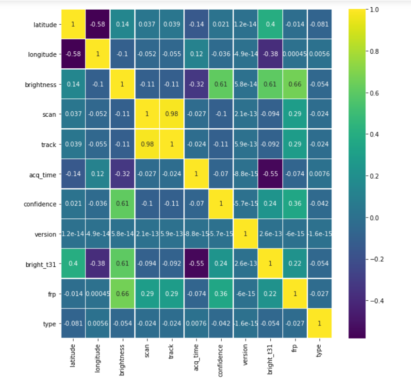
plt.figure(figsize=(10, 10))
sns.heatmap(forest.corr(),annot=True,cmap='viridis',linewidths=.5)
Output:

Data cleaning
forest = forest.drop(['track'], axis = 1)
Here we are dropping the track column
Note: By the way from the dataset we are not finding if the forest fire happens or not, we are trying to find the confidence of the forest fire happening. They may seem to be the same thing but there is a very small difference between them, try to find that 🙂
Finding categorical data
print("The scan column")
print(forest['scan'].value_counts())
print()
print("The aqc_time column")
print(forest['acq_time'].value_counts())
print()
print("The satellite column")
print(forest['satellite'].value_counts())
print()
print("The instrument column")
print(forest['instrument'].value_counts())
print()
print("The version column")
print(forest['version'].value_counts())
print()
print("The daynight column")
print(forest['daynight'].value_counts())
print()
Output:
The scan column
1.0    8284
1.1    6000
1.2    3021
1.3    2412
1.4    1848
1.5    1610
1.6    1451
1.7    1281
1.8    1041
1.9     847
2.0     707
2.2     691
2.1     649
2.3     608
2.5     468
2.4     433
2.8     422
3.0     402
2.7     366
2.9     361
2.6     347
3.1     259
3.2     244
3.6     219
3.4     203
3.3     203
3.8     189
3.9     156
4.7     149
4.3     137
3.5     134
3.7     134
4.1     120
4.6     118
4.5     116
4.2     108
4.0     103
4.4     100
4.8      70
Name: scan, dtype: int64

The aqc_time column
506     851
454     631
122     612
423     574
448     563
       ...
1558      1
635       1
1153      1
302       1
1519      1
Name: acq_time, Length: 662, dtype: int64

The satellite column
Aqua     20541
Terra    15470
Name: satellite, dtype: int64

The instrument column
MODIS    36011
Name: instrument, dtype: int64

The version column
6.3    36011
Name: version, dtype: int64

The daynight column
D    28203
N     7808
Name: daynight, dtype: int64
From the above data, we can see that some columns have just one value recurring in them, meaning they are not valuable to us
So we will drop them altogether.
Thus only satellite and day-night columns are the only categorical type.
Having said that, we can even use the scan column to restructure it into a categorical data type column. Which we will be doing in just a while.
forest = forest.drop(['instrument', 'version'], axis = 1)
forest.head()
Output:

daynight_map = {"D": 1, "N": 0}
satellite_map = {"Terra": 1, "Aqua": 0}

forest['daynight'] = forest['daynight'].map(daynight_map)
forest['satellite'] = forest['satellite'].map(satellite_map)
forest.head()
Output:

Looking at the type of another column
forest['type'].value_counts()
Output:
0    35666
2      335
3       10
Name: type, dtype: int64
Concatenating forest and types data frame
types = pd.get_dummies(forest['type'])
forest = pd.concat([forest, types], axis=1)
forest = forest.drop(['type'], axis = 1)
forest.head()
Output:

Renaming columns for better understanding
forest = forest.rename(columns={0: 'type_0', 2: 'type_2', 3: 'type_3'})
Binning Method
- Now I mentioned we will be converting scan column to categorical type, we will be doing this using the binning method.
- The range for these columns was 1 to 4.8
bins = [0, 1, 2, 3, 4, 5]
labels = [1,2,3,4,5]
forest['scan_binned'] = pd.cut(forest['scan'], bins=bins, labels=labels)
forest.head()
Output:

Converting the datatype to datetype from string or NumPy.
forest['acq_date'] = pd.to_datetime(forest['acq_date'])
Now we will be dropping the scan column and handle datetype data – we can extract useful information from these datatypes just like we do with categorical data.
forest = forest.drop(['scan'], axis = 1)
Creating a new column year with the help of acq_date column
forest['year'] = forest['acq_date'].dt.year
forest.head()
Output:

As we have added the year column similarly we will add the month and day column
forest['month'] = forest['acq_date'].dt.month
forest['day'] = forest['acq_date'].dt.day
Checking the shape of the dataset again
forest.shape
Output:
(36011, 17)
Now, as we can see that two more columns have been added which are a breakdown of date columns
Separating our target variable
y = forest['confidence']
fin = forest.drop(['confidence', 'acq_date', 'acq_time', 'bright_t31', 'type_0'], axis = 1)
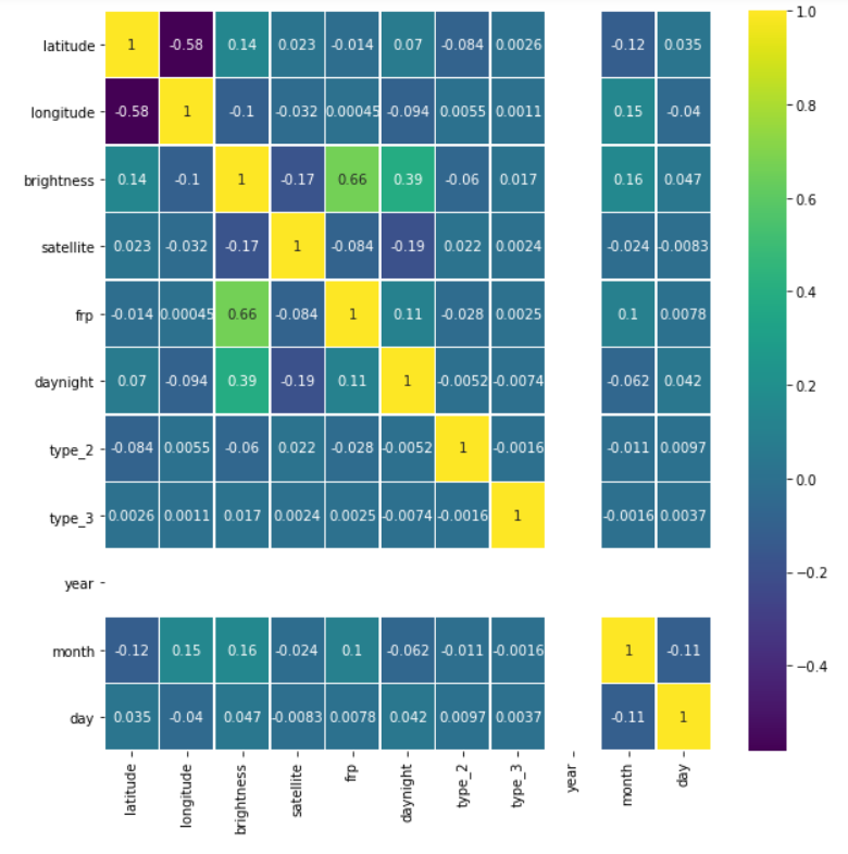
Checking for correlation once again
plt.figure(figsize=(10, 10))
sns.heatmap(fin.corr(),annot=True,cmap='viridis',linewidths=.5)
Output:

Let’s see our cleaned and sorted dataset now
fin.head()
Output:

Splitting the clean data into training and testing dataset
Xtrain, Xtest, ytrain, ytest = train_test_split(fin.iloc[:, :500], y, test_size=0.2)
Model building
Using RandomForestRegressor for model building
random_model = RandomForestRegressor(n_estimators=300, random_state = 42, n_jobs = -1)
#Fit
random_model.fit(Xtrain, ytrain)

y_pred = random_model.predict(Xtest)

#Checking the accuracy
random_model_accuracy = round(random_model.score(Xtrain, ytrain)*100,2)
print(round(random_model_accuracy, 2), '%')
Output:
95.32 %
Checking the accuracy
random_model_accuracy1 = round(random_model.score(Xtest, ytest)*100,2)
print(round(random_model_accuracy1, 2), '%')
Output:
65.32 %
Saving the model by pickle module using the serialized format
import pickle
saved_model = pickle.dump(random_model, open('ForestModelOld.pickle','wb'))
Model Tuning
- The accuracy is not so great, plus the model is overfitting
- So we use RandomCV
Getting all the parameters from the model
random_model.get_params()
Output:
{'bootstrap': True,
 'ccp_alpha': 0.0,
 'criterion': 'mse',
 'max_depth': None,
 'max_features': 'auto',
 'max_leaf_nodes': None,
 'max_samples': None,
 'min_impurity_decrease': 0.0,
 'min_impurity_split': None,
 'min_samples_leaf': 1,
 'min_samples_split': 2,
 'min_weight_fraction_leaf': 0.0,
 'n_estimators': 300,
 'n_jobs': -1,
 'oob_score': False,
 'random_state': 42,
 'verbose': 0,
 'warm_start': False}
Putting RadomizedSearchCV in action!
"""
n_estimators = number of trees in the forest
max_features = max number of features considered for splitting a node
max_depth = max number of levels in each decision tree
min_samples_split = min number of data points placed in a node before the node is split
min_samples_leaf = min number of data points allowed in a leaf node
bootstrap = method for sampling data points (with or without replacement)
"""
from sklearn.model_selection import RandomizedSearchCV
Number of trees in random forest
n_estimators = [int(x) for x in np.linspace(start = 300, stop = 500, num = 20)]
Number of features to consider at every split
max_features = ['auto', 'sqrt']
Maximum number of levels in tree
max_depth = [int(x) for x in np.linspace(15, 35, num = 7)]
max_depth.append(None)
Minimum number of samples required to split a node
min_samples_split = [2, 3, 5]
Minimum number of samples required at each leaf node
min_samples_leaf = [1, 2, 4]
Create the random grid
random_grid = {'n_estimators': n_estimators,
               'max_features': max_features,
               'max_depth': max_depth,
               'min_samples_split': min_samples_split,
               'min_samples_leaf': min_samples_leaf,
                }
print(random_grid)
Output:
{'n_estimators': [300, 310, 321, 331, 342, 352, 363, 373, 384, 394, 405, 415, 426, 436, 447, 457, 468, 478, 489, 500], 'max_features': ['auto', 'sqrt'], 'max_depth': [15, 18, 21, 25, 28, 31, 35, None], 'min_samples_split': [2, 3, 5], 'min_samples_leaf': [1, 2, 4]}
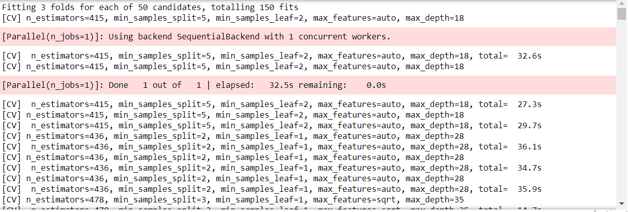
- A random search of parameters, using 3 fold cross-validation, search across 100 different combinations and use all available cores
- n_iter, which controls the number of different combinations to try, and cv which is the number of folds to use for cross-validation
rf_random = RandomizedSearchCV(estimator = random_model, param_distributions = random_grid,
                                n_iter = 50, cv = 3, verbose=2, random_state=42)
# Fit the random search model
rf_random.fit(Xtrain, ytrain)
Output:

Just like this snippet, there will be numerous folds in this RandomizedSearchCV
Getting the best parameter out of it
rf_random.best_params_
Output:
{'n_estimators': 394,
 'min_samples_split': 2,
 'min_samples_leaf': 1,
 'max_features': 'sqrt',
 'max_depth': 25}
Creating a new model with tuned parameters
random_new = RandomForestRegressor(n_estimators = 394, min_samples_split = 2, min_samples_leaf = 1, max_features = 'sqrt',
                                      max_depth = 25, bootstrap = True)
#Fit
random_new.fit(Xtrain, ytrain)
y_pred1 = random_new.predict(Xtest)
#Checking the accuracy
random_model_accuracy1 = round(random_new.score(Xtrain, ytrain)*100,2)
print(round(random_model_accuracy1, 2), '%')
Output:
95.31 %
Checking the accuracy
random_model_accuracy2 = round(random_new.score(Xtest, ytest)*100,2)
print(round(random_model_accuracy2, 2), '%')
Output:
67.39 %
Saving the tuned model by pickle module using the serialized format
saved_model = pickle.dump(random_new, open('ForestModel.pickle','wb'))
Loading the tuned pickled model
reg_from_pickle = pickle.load(saved_model)
bz2file
Here comes the cherry on the cake part (bonus of this article). Let’s understand what this bz2file module is all about. Let’s get started!
What is bz2file
bz2file is one of the modules in python which are responsible for compression and decompression of files, hence it can help in decreasing the serialized or deserialized file to a smaller size which will be very helpful in the long run when we have large datasets
How bz2file is helpful here?
As we know that our dataset is 2.7+ MB and our Random forest model is whooping 700+ MB so we need to compress that so that that model won’t be leading as a hectic situation for storage.
How to install bz2file?
- Jupyter notebook: !pip install bz2file
- Anaconda prompt/CMD: pip install bz2file
Hence I installed bz2file, which is used to compress data. This is a life-saving package for those who have low spaces on their disk but want to store or use large datasets. Now the pickled file was over 700 MB in size which when used bz2 compressed into a file of size 93 MB or less.
import bz2

compressionLevel = 9
source_file = 'ForestModel.pickle' # this file can be in a different format, like .csv or others...
destination_file = 'ForestModel.bz2'

with open(source_file, 'rb') as data:
    tarbz2contents = bz2.compress(data.read(), compressionLevel)

fh = open(destination_file, "wb")
fh.write(tarbz2contents)
fh.close()
This code will suppress the size of the tuned pickle model.
Okay so that’s a wrap from my side!
Endnotes
Thank you for reading my article 🙂
I hope you guys will like this step-by-step learning of forest fire prediction using machine learning. One last thing I wanna mention is that I’m very well aware of the fact that the accuracy of the model is not that good but the objective of the article is quite balanced so you guys can try out different Ml algorithms to look for better accuracy.
Here’s the repo link to this article.
Here you can access my other articles which are published on Analytics Vidhya as a part of the Blogathon (link)
If got any queries you can connect with me on LinkedIn, refer to this link
About me
Greeting to everyone, I’m currently working in TCS and previously I worked as a Data Science Associate Analyst in Zorba Consulting India. Along with full-time work, I’ve got an immense interest in the same field i.e. Data Science along with its other subsets of Artificial Intelligence such as, Computer Vision, Machine learning, and Deep learning feel free to collaborate with me on any project on the above-mentioned domains (LinkedIn).
Image Source-
- Image 1 – https://www.theleader.info/wp-content/uploads/2017/08/forest-fire.jpg


Very nice your post. But what will be the final outcome of the code?
Hello the post has been very much helpful to me but I want to know more about data sets? Like from where the data sets have been taken, as per the normal data set for the forest fire prediction conclude fwi, ffmc etc. but here nothing aligns.. So please help me I will grateful for your help
hi, can you please provide me the dataset link