This article was published as a part of the Data Science Blogathon
A comprehensive guide for finding the best hyper-parameter for your model efficiently.
Tuning hyperparameter is more efficient with Bayesian optimized algorithms compared to Brute-force algorithms.
You will see how to find the best hyperparameters for XGboost Regressor in this article.
Introduction
Optimizing ML models is a very challenging job. There are many tools in the market that makes our fine-tuning easier, In order to optimize our model, you need to make sure that our data is meaningful and our ML model fits on it perfectly. In this article, we will see how to fine-tune an Xgboost regressor in the easiest way possible.
In machine learning, a hyperparameter is a parameter whose value is used to control the learning process. ie-LR, regularization, gamma, and so on. Hyperparameters’ values can’t be estimated from the data. These are parameters that control the learning of the model on our data.
You can control the learning parameters in-order to make the model perfectly fit and learn from our data and give skilful predictions. Hyperparameter optimization of ML models gets complicated as our model gets complex. there are some popular ways to find optimized hyperparameters.
- Grid Search: Grid Search trains the model on all possible hyperparameter combination and then compare using cross-validation.
- Randomized Search: Randomized Search trains a model on a random hyperparameter combination and then compares using cross-validation.
- Bayesian approach: it uses the Bayesian technique to model the search space and to reach an
optimized parameter. There are many handy tools designed for fast
hyperparameter optimization for complex deep learning and ML models like
HyperOpt, Optuna, SMAC, Spearmint, etc.
Optuna
Optuna is the SOTA algorithm for fine-tuning ML and deep learning models. It depends on the Bayesian fine-tuning technique. It prunes unpromising trials which don’t further improve our score and try only that combination that improves our score overall.
Salient Features of Optuna:
- Efficiently search large spaces and prune unpromising trials for faster results.
- Parallelize hyperparameter searches over multiple threads or processes without modifying code.
- Automated search for optimal hyperparameters using Python conditionals, loops, and syntax.
Tuning Process using Optuna
Article Checkpoints:
- Train Xgboost on the boston_housing dataset.
- Explore hyperparameter tuning in detail.
- Analyze the visualization for better and faster tuning.
Load the Data and Libraries
Importing necessary modules and loading the data into a data frame.
import sklearn
import pandas as pd
import numpy as np
from sklearn.datasets import load_boston
boston = load_boston()
df = pd.DataFrame(boston.data , columns = boston.feature_names)
df['target'] = boston.target
X = df.iloc[:,df.columns != 'target']
y = df.target
load_boston() returns the data in matrix form and after framing it into pandas data frame we separated X (features), y (target).
from sklearn.preprocessing import StandardScaler
se = StandardScaler()
X = se.fit_transform(X)
Scaling the dataset into one scale, helps the model to converge efficiently and split the dataset into train and test.
from sklearn.model_selection import train_test_split
X_train, X_test, y_train,y_test = train_test_split(X, y, test_size = 0.2, random_state = 12)
Before Tuning First Test the Base Model
Building a Vanilla (default) model before gives a scale for comparison,
and we can compare how much our model has improved after parameter
fine-tuning.
import xgboost as xgb
from sklearn.model_selection import cross_val_score
xg_reg = xgb.XGBRegressor()
scores = cross_val_score(xg_reg, X_train,y_train , scoring = 'neg_root_mean_squared_error',n_jobs = -1,cv = 10)
print(np.mean(scores), np.std(scores))
print(scores)

for some reason cross_val_score has “neg_root_mean_squared_error”, we can change this into positive by multiplying by -1.
- cross_val_score Evaluate a score by cross-validation.
KFoldcreates a custom k cross-validation.- here scoring is “root_mean_squared_error” lower is better.
- cv = 10 folds , n_jobs= -1 ( using all available CPUs).
Define Function that Takes Hyper-Parameters and Return Scores
We often calculate rmse in the regressor model and AUC scores for the classifier model.
def return_score(param):
  model = xgb.XGBRegressor(**param)
  rmse = -np.mean(model_selection.cross_val_score(model,X_train[:1000],y_train[:10000], cv = 4, n_jobs =-1,scoring='neg_root_mean_squared_error'))
  return rmse
return_score() takes parameters as keyword argument and returns the cross_validated value for -(neg_root_mean_squared_error), in order to save time, we are taking only 1000 samples.
Import Optuna
This is the step where actual Optuna comes into the Picture.
import optuna
from optuna import Trial, visualization
from optuna.samplers import TPESampler
- Samplers class provides us with a class to define our hyper-parameter space.
- Visualization is used to plot the tuning results.
- A trial is a method of determining the effectiveness of an objective function.
Creating Hyper-Parameters Space
Time to create our main objective function, we put all the possible
hyper-parameter ranges and the function takes a trial object and should
return a score value.
We have various ways to define the ranges of possible hyper-parameter values:-
- trial.suggest_uniform(‘reg_lambda’,0,2)
- trial.suggest_int(‘ParamName’, 2 , 5)
- trial.suggest_loguniform(‘learning_rate’,0.05,0.5)
def objective(trial):
  param = {
                "n_estimators" : trial.suggest_int('n_estimators', 0, 500),
                'max_depth':trial.suggest_int('max_depth', 3, 5),
                'reg_alpha':trial.suggest_uniform('reg_alpha',0,6),
                'reg_lambda':trial.suggest_uniform('reg_lambda',0,2),
                'min_child_weight':trial.suggest_int('min_child_weight',0,5),
                'gamma':trial.suggest_uniform('gamma', 0, 4),
                'learning_rate':trial.suggest_loguniform('learning_rate',0.05,0.5),
                'colsample_bytree':trial.suggest_uniform('colsample_bytree',0.4,0.9),
                'subsample':trial.suggest_uniform('subsample',0.4,0.9),
                'nthread' : -1
            }
  return(return_score(param)) # this will return the rmse score
For A detailed explanation on various parameters refer to this link.
Start Tuning
In order to start our searching of hyperparameters, we need to first create an optuna– study object, which holds all the information of hyper-parameters tried under that study.
The study creates an object which holds all the parameters, history about that particular optimization.
study1 = optuna.create_study(direction='minimize',sampler=TPESampler())
study1.optimize(objective, n_trials= 550,show_progress_bar = True)
- direction = ‘minimize’,
rmse. - show_progress_bar = True, gives a nice-looking progress bar.
- n_trails = 1050, is the same as the epoch.
- sampler = TPESample(), Bayesian Sampling Technique
Let’s Run the study !!
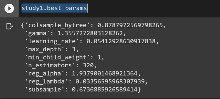
After 1050 trials we got our best hyper-parameters as shown below

In the beginning, we had rmse 2.98 and after 500 trials it became 2.54.
How to get tuned hyper-parameters?
The study object holds all the information of the particular search.
Calling study.best_params returns the optimized parameters in the form of a dictionary.
study1.best_params

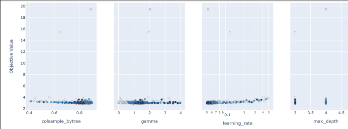
Visualization of Tuning
Visualizing search history gives us a better idea of the effect of
hyper-parameters on our model. we can also further narrow down the
search by using narrower parameters space.
optuna.visualization.plot_slice(study1)

These are the values of various hyper-parameters and their impact on our objective value (rmse in this case)
from the above graph, the minimum rmse found when max_depth was 3, learning_rate was .054, n_estimators = 340, and so on…
We can further deep dive and try to tune using narrower range of hyper-parameters values by taking help of visualizations.
Compare the Tuned Model and Base Model
Let’s see how much our model has improved.
params = {}
print(f"without tuning {return_score(params)}")
print(f"with tuning {return_score(study1.best_params)}")
For the default model, we are not specifying any hyperparameters, the model will be using the default hyper-parameters, for the Optimized model we are passing study1.best_params which returns the optimized h-parameters in a form of a dictionary.

Perfect !! as you can see after fine-tuning we have got a lower rmse by 30 units. It does not end, we can fine-tune further-more by narrowing the hyperparameters ranges.
Conclusion
In this article we have seen how to optimize ML models, we saw how to find optimized parameters, but this is not the end. you can improve it further by narrowing down the learning parameter ranges.
In the next article, we will learn fine-Tuning of Xgboost Classifier using HyperOpt
Download full Code here.
Thanks for reading the article, please share if you liked this article.
Article From: Abhishek Jaiswal, Reach out to me on LinkedIn.


