This article was published as a part of the Data Science Blogathon.
Table of contents
- Introduction
- Confidence Intervals with Z-statistic
- Interpreting Confidence Intervals
- Assumptions for CI using z-statistic
- Confidence intervals with t-statistic
- Assumptions for CI using t-statistic
- Making a t-interval with paired data
- z-value vs t-value: when to use what?
- Confidence Intervals with python
- End-Note
Introduction
Whenever we solve a statistical problem we are concerned about the estimation of population parameters but more often than not it is close to impossible to calculate population parameters. What we do instead is take random samples from the population and calculate sample statistics expecting to approximate population parameters. But how do we know if the samples are true representatives of the population or how much these sample statistics deviate from population parameters? This is where confidence intervals come into the picture. So, what these intervals are? The confidence interval is a range of values ranging above and below the sample statistics or we can also define it as the probability that a range of values around the sample statistic contains the true population parameter.
Confidence Intervals with Z-statistic
Before delving deep into the topic let’s get acquainted with some statistical terminologies.
population: It is the set of all similar individuals. For example the population of a city, students of a college, etc.
sample: It is a small set of similar individuals drawn from the population. Similarly, a random sample is a sample drawn at random from the population.
parameters: Mean(mu), standard deviations(sigma), proportion(p) derived from the population.
statistic: mean(x bar), std deviation(S), proportions(p^) concerned with samples.
Z-score: it is the distance of any raw data point on a normal distribution from the mean normalized by std deviation. Given by: x-mu/sigma
All right now we are ready to dive deep into the concept of confidence intervals. For some reason, I believe it is much better to understand concepts through relatable examples rather than raw mathematical definitions. So let’s get started.
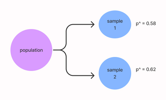
suppose, you live in a city of population 100,000 and an election is around the corner. As a pollster, you must forecast who is going to win the election either blue party or yellow. So, you see it is almost impossible to collect information from the entire population so you randomly pick 100 people. At the end of the survey, you found that 62% of people are going to vote for yellow. Now the question is should we conclude that yellow is going to win with a win probability of 62% or 62% of the entire population will be voting for yellow? Well, the answer is NO. We don’t know for sure how far our estimation is from the true parameter, if we take another sample the result may turn out to be 58% or 65%. So, what we will do instead is to find a range of values around our sample statistic that will most likely capture the true population proportion. Here, the proportion refers to the percentage of people voting yellow.

image belongs to the author
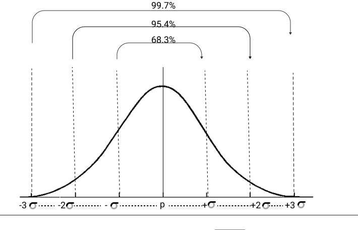
Now, if we take a hundred such samples and plot the sample proportion of each sample we will get a normal distribution of sampling proportions and the mean of the distribution will be the most approximate value of the population proportion. And our estimate could lie anywhere on the distribution curve. As per the 3-sigma rule, we know that around 95% of the random variables lie within 2 std deviations from the mean of the distribution. So, we can conclude that the probability that p^ is within 2 std deviations of p is 95%. Or we can also state that the probability that p is within 2 std deviations below and above p^ is also 95%. These two statements are effectively equivalent. These two points below and above the p^ are our confidence intervals.

image belongs to the author
If we can somehow find the sigma we can calculate our required interval. But sigma here is the population parameter and we know it is often near impossible to calculate so instead we will use sample statistics i.e. Standard error. This is given as
where p^= sample proportion, n=number of samples
SE =√(0.62 . 0.38/100) = 0.05
so, 2xSE = 0.1
Confidence interval for our data is (0.62-0.1,0.62+0.1) or (0.52,0.72). As we have taken 2xSE this translates to 95% confidence interval.
Now, the question is what if we want to create a 92% confidence interval? In the previous example, we multiplied 2 with SE to construct a 95% confidence interval, this 2 is the z-score for a 95% confidence interval (exact value being 1.96) and this value can be found from a z-table. The critical value of z for a 92% confidence interval is 1.75. Refer to this article for a better understanding of z-score and z-table.
The interval is given by: (p^ + z*.SE , p^-z*.SE).
If instead of sample proportion sample mean is given the standard error will be sigma/sqrt(n). Here sigma is the population std deviation as we often don’t have we use sample std deviation instead. But it is often observed that this kind of estimation where the mean is given the result tends to be a bit biased. So in cases like this, it is preferred to use t-statistic instead of z-statistics.
The general formula for a confidence interval with z-statistics is given by
Here, the statistic refers to either sample mean or sample proportion. sigmas are the population standard deviation.
Interpreting Confidence Intervals
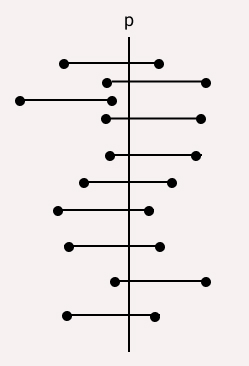
It is really important to interpret confidence intervals correctly. Consider the previous pollster example where we calculated our 95% confidence interval to be (0.52,0.62). What does that mean? Well, a 95% confidence interval means if we draw n samples from the population then 95% of the time the derived interval will contain the true population proportion. Remember a 95% confidence interval does not mean that there’s a 95% probability that the interval contains the true population proportion. For example, for a 90% confidence interval if we draw 10 samples from a population then 9 out of 10 times the said interval will contain true population parameter. Look at the below picture for a better understanding.

image belongs to the author
Assumptions for confidence intervals using Z-statistic
There are certain assumptions we need to look for to construct a valid confidence interval using z-statistic.
- Random sample: The samples need to be random. There are different sampling methods like stratified sampling, simple random sampling, cluster sampling to get random samples.
- Normal condition: The data must satisfy this condition n.p^>=10 and n.(1-p^)>=10. That essentially means is our sampling distribution of sample means needs to be normal, not skewed on either side.
- Independent: The samples need to be independent. The number of samples needs to be less than or equal to 10% of the total population or if the sampling is done with replacement.
Confidence Intervals with T-statistic
What if the sample size is relatively small and the population standard deviation isn’t given or cannot be assumed? How do we construct a confidence interval? well, that is where t-statistic comes in. The basic formula for finding confidence interval here remains the same with just z* replaced by t*. The general formula is given by
where S = sample standard deviation, n = number of samples
Suppose, you hosted a party and you want to estimate the average consumption of beer by your guests. So, you obtain a random sample of 20 individuals and measured the beer consumption. The sample data is symmetric with a mean 0f 1200 ml and std deviation of 120 ml. So, now you wish to construct a 95% confidence interval.
So, we have sample std deviation, the number of samples, and sample mean. All we need is t*. So, t* for a 95% confidence interval with a degree of freedom of 19(n-1 = 20-1) is 2.093. So, our required interval is after the calculation is (1256.16, 1143.83) with a margin of error of 56.16. Refer to this video to know how to read the t-table.
Assumtions for CI using T-statistic
Similar to the case of z-statistic here in the case of t-statistic too there are some conditions we need to look out for in given data.
- The sample needs to be random
- The sample needs to be normal. To be normal the sample size should be greater or equal to 30 or if the parent dataset i.e. the population is roughly normal. Or if the sample size is below 30 then the distribution needs to be roughly symmetric.
- Individual observations need to be independent. That means it follows the 10% rule or sampling is done with replacement.
Making a T-interval for paired data
Until now we have only used one-sample data. Now we will see how we can construct a t-interval for paired data. In paired data, we make two observations on the same individual. For example, comparing pre-test and post-test marks of students or data on the effect of a drug and placebo on a group of persons. In paired data, we found the difference between the two observations in the 3rd column. As usual, we will go through an example to understand this concept as well,
Q. A teacher tried to evaluate the effect of a new curriculum on the test result. Below are the results of the observations.
.jpg)
image belongs to the author
As we intend to find intervals for the mean difference, we only need the statistics for the differences. We will use the same formula that we used before
statistic +- (critical value or t-value) (standard deviation of statistic)
xd = mean of difference, Sd = sample std deviation, for a 95% CI with a degree of freedom 5 t* is given by 2.57. The margin of error = 0.97 and the confidence interval (4.18,6.13).
Interpretation: From the above estimates as we can see the confidence interval does not contain zero or negative values. So, we can conclude that the new curriculum had a positive impact on the test performances of students. If it had only negative values then we could say that the curriculum had a negative impact. Or if it contained zero then there could be a possibility that the difference was zero or no effect of curriculum on test results.
Z-value vs T-value
There’s a lot of confusion at the beginning about when to use what. The rule of thumb is when the sample size is >= 30 and population standard deviation is known to use z-statistics. In case the sample size is < 30 use t-statistics. In real life, we don’t have population parameters so we will go with z or t based on sample size.
With smaller samples(n<30) the central LImit Theorem does not apply, and another distribution called Student’s t-distribution is used. The t-distribution is similar to normal distribution but takes different shapes depending on the sample size. Instead of z values, t values are used which are larger for smaller samples, producing a larger margin of error. As a small sample size will be less precise.
Confidence Intervals with Python
Python has a vast library supporting all kinds of statistical calculations making our life a bit easier. In this section, we will look at the data on toddlers’ sleep habits. The 20 participants of these observations were healthy, normal behaved, not have any sleeping disorder. Our goal is to analyze the bedtime of napping and non-napping toddlers.
Reference: Akacem LD, Simpkin CT, Carskadon MA, Wright KP Jr, Jenni OG, Achermann P, et al. (2015) The Timing of the Circadian Clock and Sleep Differ between Napping and Non-Napping Toddlers. PLoS ONE 10(4): e0125181. https://doi.org/10.1371/journal.pone.0125181
We will be importing libraries that we will need
import numpy as np
import pandas as pd
from scipy.stats import t
pd.set_option('display.max_columns', 30) # set so can see all columns of the DataFrame
import math
df = pd.read_csv(nap_no_nap.csv) #reading data
df.head()
.png)
Create two 95% confidence intervals for the average bedtime, one for toddlers who nap and one for toddlers who don’t. First, we will isolate the column ‘night bedtime’ for those who nap into a new variable, and those who didn’t nap into another new variable. The bedtime here is decimalized.
bedtime_nap = df['night bedtime'].loc[df['napping'] == 1]
bedtime_no_nap = df['night bedtime'].loc[df['napping'] == 0]
output: 15 n 5
Now, we will find the sample mean bedtime for nap and no_nap.
nap_mean_bedtime = bedtime_nap.mean() #20.304
no_nap_mean_bedtime = bedtime_no_nap.mean() #19.59
Now, we will find the sample standard deviation for Xnap and Xno nap
nap_s_bedtime = np.std(bedtime_nap,ddof=1)
no_nap_s_bedtime = np.std(bedtime_no_nap,ddof=1)
Note: The ddof parameter is set to 1 for sample std dev or else it will become population std dev.
Now, we will find the sample standard error for Xnap and Xno nap
nap_se_mean_bedtime = nap_s_bedtime/math.sqrt(len(bedtime_nap)) #0.1526
no_nap_se_mean_bedtime = no_nap_s_bedtime/math.sqrt(len(bedtime_no_nap)) #0.2270
So far so good, now as the sample size is small and we do not have a standard deviation of population proportion we will use the t* value. One way to find the t* value is by using scipy.stats t.ppf function. The arguments for t.ppf() are q = percentage, df = degree of freedom, scale = std dev, loc = mean. As t-distribution is symmetric for a 95% confidence interval q will be 0.975. Refer to this for more info on t.ppf().
nap_t_star = t.ppf(0.975,df=14) #2.14
no_nap_t_star = t.ppf(0.975,df=5) #2.57
Now, we will add the pieces to finally construct our confidence interval.
output: 19.976680775477412 20.631319224522585
18.95974084563192 20.220259154368087
Interpretation:
From the above results, we conclude that we are 95% confident that the average bedtime for napping toddlers is between the time 19.98 – 20.63 (pm) while for non-napping toddlers it is between 18.96 – 20.22 (pm). These results are as per our expectation that if you take a nap during the day you will sleep late at night.
EndNotes
So, this was all about simple confidence intervals using z and t values. It is indeed an important concept to know in the case of any statistical study. A great inferential statistical method to estimate population parameters from sample data. Confidence intervals are also linked to hypothesis testing that for a 95% CI you leave 5% space for anomalies. If the null hypothesis falls within the confidence interval then the p-value will be large and we will not be able to reject null. Conversely, if it falls beyond then we will have sufficient proof to reject null and accept alternate hypotheses.
Hope you liked the article and Happy new year (:
The media shown in this article is not owned by Analytics Vidhya and are used at the Author’s discretion.


