This article was published as a part of the Data Science Blogathon.
Introduction
Technology is evolving round the clock in recent times. This has resulted in job opportunities for people all around the world. It comes with a hectic schedule that can be detrimental to people’s mental health. So During the Covid-19 pandemic, mental health has been one of the most prominent issues, with stress, loneliness, and depression all on the rise over the last year. Diagnosing mental health is difficult because people aren’t always willing to talk about their problems.
Machine learning is a branch of artificial intelligence that is mostly used nowadays. ML is becoming more capable for disease diagnosis and also provides a platform for doctors to analyze a large number of patient data and create personalized treatment according to the patient’s medical situation.
In this article, we are going to predict the mental health of Employees using various machine learning models. You can download the dataset from this link.
Library and Data Loading
import numpy as np
import pandas as pd
import matplotlib.pyplot as plt
import seaborn as sns
from scipy import stats
from scipy.stats import randint
# prep
from sklearn.model_selection import train_test_split
from sklearn import preprocessing
from sklearn.datasets import make_classification
from sklearn.preprocessing import binarize, LabelEncoder, MinMaxScaler
# models
from sklearn.linear_model import LogisticRegression
from sklearn.tree1 import DecisionTreeClassifier
from sklearn.ensemble import RandomForestClassifier, ExtraTreesClassifier
# Validation libraries
from sklearn import metrics
from sklearn.metrics import accuracy_score, mean_squared_error, precision_recall_curve
from sklearn.model_selection import cross_val_score1
#Neural Network
from sklearn.neural_network import MLPClassifier
from sklearn.model_selection import RandomizedSearchCV
#Bagging
from sklearn.ensemble import BaggingClassifier, AdaBoostClassifier
from sklearn.neighbors import KNeighborsClassifier
#Naive bayes
from sklearn.naive_bayes import GaussianNB
#Stacking
from mlxtend.classifier import StackingClassifier
from google.colab import files
uploaded = files.upload()
train_df = pd.read_csv('survey.csv')
print(train_df.shape)
print(train_df.describe())
print(train_df.info())
(1259, 27)
Age
count 1.259000e+03
mean 7.942815e+07
std 2.818299e+09
min -1.726000e+03
25% 2.700000e+01
50% 3.100000e+01
75% 3.600000e+01
max 1.000000e+11
RangeIndex: 1259 entries, 0 to 1258
Data columns (total 27 columns):
# Column Non-Null Count Dtype
— —— ————– —–
0 Timestamp 1259 non-null object
1 Age 1259 non-null int64
2 Gender 1259 non-null object
3 Country 1259 non-null object
4 State 744 Non-null object
5 self_employed 1241 non-null object
6 family_history 1259 non-null object
7 treatment 1259 non-null object
8 work_interfere 995 non-null object
9 no_employees 1259 non-null object
10 remote_work 1259 non-null object
11 tech_company 1259 non-null object
12 benefits 1259 non-null object
13 care_options 1259 non-null object
14 wellness_program 1259 non-null object
15 seek_help 1259 non-null object
16 anonymity 1259 non-null object
17 leave 1259 non-null object
18 mental_health_consequence 1259 non-null object
19 phys_health_consequence 1259 non-null object
20 coworkers 1259 non-null object
21 Supervisor 1259 non-null object
22 mental_health_interview 1259 non-null object
23 phys_health_interview 1259 non-null object
24 mental_vs_physical 1259 non-null object
25 obs_consequence 1259 non-null object
26 comments 164 non-null object
dtypes: int64(1), object(26)
memory usage: 265.7+ KB
None
Data Cleaning
#missing data
total = train_df.isnull().sum().sort_values(ascending=False)
percent = (train_df.isnull().sum()/train_df.isnull().count()).sort_values(ascending=False)
missing_data = pd.concat([total, percent], axis=1, keys=['Total', 'Percent'])
missing_data.head(20)
print(missing_data)
Total Percent
comments 1095 0.869738
state 515 0.409055
work_interfere 264 0.209690
self_employed 18 0.014297
benefits 0 0.000000
Age 0 0.000000
Gender 0 0.000000
Country 0 0.000000
family_history 0 0.000000
treatment 0 0.000000
no_employees 0 0.000000
remote_work 0 0.000000
tech_company 0 0.000000
care_options 0 0.000000
obs_consequence 0 0.000000
wellness_program 0 0.000000
seek_help 0 0.000000
anonymity 0 0.000000
leave 0 0.000000
mental_health_consequence 0 0.000000
phys_health_consequence 0 0.000000
coworkers 0 0.000000
Supervisor 0 0.000000
mental_health_interview 0 0.000000
phys_health_interview 0 0.000000
mental_vs_physical 0 0.000000
Timestamp 0 0.000000
#dealing with missing data
train_df.drop(['comments'], axis= 1, inplace=True)
train_df.drop(['state'], axis= 1, inplace=True)
train_df.drop(['Timestamp'], axis= 1, inplace=True)
train_df.isnull().sum().max() #just checking that there's no missing data missing...
train_df.head(5)

defaultInt = 0
defaultString = 'NaN'
defaultFloat = 0.0
# Create lists by data tpe
intFeatures = ['Age']
floatFeatures = []
# Clean the NaN's
for feature in train_df:
    if feature in intFeatures:
        train_df[feature] = train_df[feature].fillna(defaultInt)
    elif feature in stringFeatures:
        train_df[feature] = train_df[feature].fillna(defaultString)
    elif feature in floatFeatures:
        train_df[feature] = train_df[feature].fillna(defaultFloat)
    else:
        print('Error: Feature %s not identified.' % feature)
train_df.head()

#Clean 'Gender'
gender = train_df['Gender'].unique()
print(gender)
#Get rid of bullshit
stk_list = ['A little about you', 'p']
train_df = train_df[~train_df['Gender'].isin(stk_list)]
print(train_df['Gender'].unique())
[‘female’ ‘male’ ‘trans’]
#complete missing age with mean
train_df['Age'].fillna(train_df['Age'].median(), inplace = True)
# Fill with media() values  120
s = pd.Series(train_df['Age'])
s[s<18] = train_df['Age'].median()
train_df['Age'] = s
s = pd.Series(train_df['Age'])
s[s>120] = train_df['Age'].median()
train_df['Age'] = s
#Ranges of Age
train_df['age_range'] = pd.cut(train_df['Age'], [0,20,30,65,100], labels=["0-20", "21-30", "31-65", "66-100"], include_lowest=True)
#There are only 0.014% of self employed so let's change NaN to NOT self_employed
#Replace "NaN" string from defaultString
train_df['self_employed'] = train_df['self_employed'].replace([defaultString], 'No')
print(train_df['self_employed'].unique())
[‘No’ ‘Yes’]
#There are only 0.20% of self work_interfere so let's change NaN to "Don't know
#Replace "NaN" string from defaultString
train_df['work_interfere'] = train_df['work_interfere'].replace([defaultString], 'Don't know' )
print(train_df['work_interfere'].unique())
[‘Often’ ‘Rarely’ ‘Never’ ‘Sometimes’ “Don’t know”]
Encoding Data
#Encoding data
labelDict = {}
for feature in train_df:
    le = preprocessing.LabelEncoder()
    le.fit(train_df[feature])
    le_name_mapping = dict(zip(le.classes_, le.transform(le.classes_)))
    train_df[feature] = le.transform(train_df[feature])
    # Get labels
    labelKey = 'label_' + feature
    labelValue = [*le_name_mapping]
    labelDict[labelKey] =labelValue
for key, value in labelDict.items():
    print(key, value)
#Get rid of 'Country'
train_df = train_df.drop(['Country'], axis= 1)
train_df.head()

#missing data
total = train_df.isnull().sum().sort_values(ascending=False)
percent = (train_df.isnull().sum()/train_df.isnull().count()).sort_values(ascending=False)
missing_data = pd.concat([total, percent], axis=1, keys=['Total', 'Percent'])
missing_data.head(20)
print(missing_data)
Total Percent
age_range 0 0.0
obs_consequence 0 0.0
Gender 0 0.0
self_employed 0 0.0
family_history 0 0.0
treatment 0 0.0
work_interfere 0 0.0
no_employees 0 0.0
remote_work 0 0.0
tech_company 0 0.0
benefits 0 0.0
care_options 0 0.0
wellness_program 0 0.0
seek_help 0 0.0
anonymity 0 0.0
leave 0 0.0
mental_health_consequence 0 0.0
phys_health_consequence 0 0.0
coworkers 0 0.0
supervisor 0 0.0
mental_health_interview 0 0.0
phys_health_interview 0 0.0
mental_vs_physical 0 0.0
Age 0 0.0
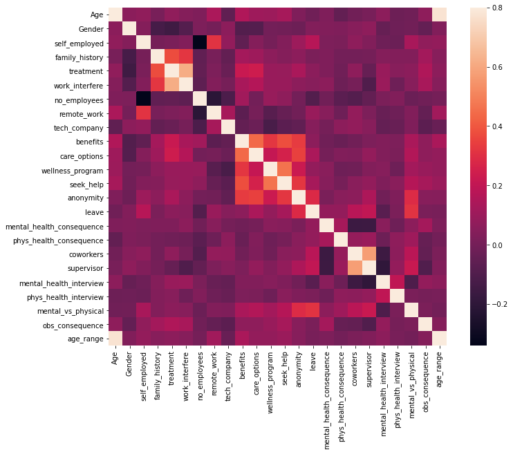
Covariance Matrix
Variability comparison between categories of variables
#correlation matrix
corrmat = train_df.corr()
f, ax = plt.subplots(figsize=(12, 9))
sns.heatmap(corrmat, vmax=.8, square=True);
plt.show()
k = 10
cols = corrmat.nlargest(k, 'treatment')['treatment'].index
cm = np.corrcoef(train_df[cols].values.T)
sns.set(font_scale=1.25)
hm = sns.heatmap(cm, cbar=True, annot=True, square=True, fmt='.2f', annot_kws={'size': 10}, yticklabels=cols.values, xticklabels=cols.values)
plt.show()
.png)
Some Charts to see the Data Relationship
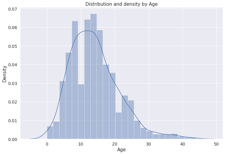
# Distribution and density by Age
plt.figure(figsize=(12,8))
sns.distplot(train_df["Age"], bins=24)
plt.title("Distribution and density by Age")
plt.xlabel("Age")
Text(0.5, 0, ‘Age’)
Inference: The above plot shows the Age column with respect to density. We can see that density is higher from Age 10 to 20 years in our dataset.
j = sns.FacetGrid(train_df, col='treatment', size=5)
j = j.map(sns.distplot, "Age")
.png)
Inference: Treatment 0 means treatment is not necessary 1 means it is. First Barplot shows that from age 0 to 10-year treatment is not necessary and is needed after 15 years.
plt.figure(figsize=(12,8))
labels = labelDict['label_Gender']
j = sns.countplot(x="treatment", data=train_df)
j.set_xticklabels(labels)
plt.title('Total Distribution by treated or not')
Text(0.5, 1.0, ‘Total Distribution by treated or not’)
.png)
Inference: Here we can see that more males are treated as compared to females in the dataset.
o = labelDict['label_age_range']
j = sns.factorplot(x="age_range", y="treatment", hue="Gender", data=train_df, kind="bar",  ci=None, size=5, aspect=2, legend_out = True)
j.set_xticklabels(o)
plt.title('Probability of mental health condition')
plt.ylabel('Probability x 100')
plt.xlabel('Age')
new_labels = labelDict['label_Gender']
for t, l in zip(j._legend.texts, new_labels): t.set_text(l)
j.fig.subplots_adjust(top=0.9,right=0.8)
plt.show()
.png)
Inference: This barplot shows the mental health of females, males, and transgender according to different age groups. we can analyze that from the age group of 66 to 100, mental health is very high in females as compared to another gender. And from age 21 to 64, mental health is very high in transgender as compared to males.
o = labelDict['label_family_history']
j = sns.factorplot(x="family_history", y="treatment", hue="Gender", data=train_df, kind="bar", ci=None, size=5, aspect=2, legend_out = True)
j.set_xticklabels(o)
plt.title('Probability of mental health condition')
plt.ylabel('Probability x 100')
plt.xlabel('Family History')
new_labels = labelDict['label_Gender']
for t, l in zip(g._legend.texts, new_labels): t.set_text(l)
j.fig.subplots_adjust(top=0.9,right=0.8)
plt.show()
.png)
o = labelDict['label_care_options']
j = sns.factorplot(x="care_options", y="treatment", hue="Gender", data=train_df, kind="bar", ci=None, size=5, aspect=2, legend_out = True)
j.set_xticklabels(o)
plt.title('Probability of mental health condition')
plt.ylabel('Probability x 100')
plt.xlabel('Care options')
new_labels = labelDict['label_Gender']
for t, l in zip(g._legend.texts, new_labels): t.set_text(l)
j.fig.subplots_adjust(top=0.9,right=0.8)
plt.show()
Inference: In the dataset, for those who are having a family history of mental health problems, the Probability of mental health will be high. So here we can see that probability of mental health conditions for transgender is almost 90% as they have a family history of medical health conditions.
.png)
Inference: This barplot shows health status with respect to care options. In the dataset, for Those who are not having care options, the Probability of mental health situation will be high. So here we can see that the mental health of transgender is very high who have not care options and low for those who are having care options.
o = labelDict['label_benefits']
j = sns.factorplot(x="care_options", y="treatment", hue="Gender", data=train_df, kind="bar", ci=None, size=5, aspect=2, legend_out = True)
j.set_xticklabels(o)
plt.title('Probability of mental health condition')
plt.ylabel('Probability x 100')
plt.xlabel('Benefits')
new_labels = labelDict['label_Gender']
for t, l in zip(j._legend.texts, new_labels): t.set_text(l)
j.fig.subplots_adjust(top=0.9,right=0.8)
plt.show()
.png)
Inference: This barplot shows the probability of health conditions with respect to Benefits. In the dataset, for those who are not having any benefits, the Probability of mental health conditions will be high. So here we can see that probability of mental health conditions for transgender is very high who have not getting any benefits. and probability is low for those who are having benefits options.
o = labelDict['label_work_interfere']
j = sns.factorplot(x="work_interfere", y="treatment", hue="Gender", data=train_df, kind="bar", ci=None, size=5, aspect=2, legend_out = True)
j.set_xticklabels(o)
plt.title('Probability of mental health condition')
plt.ylabel('Probability x 100')
plt.xlabel('Work interfere')
new_labels = labelDict['label_Gender']
for t, l in zip(g._legend.texts, new_labels): t.set_text(l)
j.fig.subplots_adjust(top=0.9,right=0.8)
plt.show()
.png)
Inference: This barplot shows the probability of health conditions with respect to work interference. For those who are not having any work interference, the Probability of mental health conditions will be very less. and probability is high for those who are having work interference rarely.
Scaling and Fitting
# Scaling Age
scaler = MinMaxScaler()
train_df['Age'] = scaler.fit_transform(train_df[['Age']])
train_df.head()

# define X and y
feature_cols1 = ['Age', 'Gender', 'family_history', 'benefits', 'care_options', 'anonymity', 'leave', 'work_interfere']
X = train_df[feature_cols1]
y = train_df.treatment
X_train1, X_test1, y_train1, y_test1 = train_test_split(X, y, test_size=0.30, Random_state1=0)
# Create dictionaries for final graph
# Use: methodDict['Stacking'] = accuracy_score
methodDict = {}
rmseDict = ()
forest = ExtraTreesClassifier(n_estimators=250,
                              Random_state1=0)
forest.fit(X, y)
importances = forest.feature_importances_
std = np.std([tree1.feature_importances_ for tree in forest.estimators_],
             axis=0)
indices = np.argsort(importances)[::-1]
labels = []
for f in Range(x.shape[1]):
    labels.append(feature_cols1[f])
plt.figure(figsize=(12,8))
plt.title("Feature importances")
plt.bar(range(X.shape[1]), importances[indices],
       color="r", yerr=std[indices], align="center")
plt.Xticks(range(X.shape[1]), labels, rotation='vertical')
plt.xlim([-1, X.shape[1]])
plt.show()
.png)
Tuning
def evalClassModel(model, y_test1, y_pred_class, plot=False):
    #Classification accuracy: percentage of correct predictions
    # calculate accuracy
    print('Accuracy:', metrics.accuracy_score(y_test1, y_pred_class))
    print('Null accuracy:n', y_test1.value_counts())
    # calculate the percentage of ones
    print('Percentage of ones:', y_test1.mean())
    # calculate the percentage of zeros
    print('Percentage of zeros:',1 - y_test1.mean())
    print('True:', y_test1.values[0:25])
    print('Pred:', y_pred_class[0:25])
    #Confusion matrix
    confusion = metrics.confusion_matrix(y_test1, y_pred_class)
    #[row, column]
    TP = confusion[1, 1]
    TN = confusion[0, 0]
    FP = confusion[0, 1]
    FN = confusion[1, 0]
    # visualize Confusion Matrix
    sns.heatmap(confusion,annot=True,fmt="d")
    plt.title('Confusion Matrix')
    plt.xlabel('Predicted')
    plt.ylabel('Actual')
    plt.show()
    accuracy = metrics.accuracy_score(y_test1, y_pred_class)
    print('Classification Accuracy:', accuracy)
    print('Classification Error:', 1 - metrics.accuracy_score(y_test1, y_pred_class))
    fp_rate = FP / float(TN + FP)
    print('False Positive Rate:', fp_rate)
    print('Precision:', metrics.precision_score(y_test1, y_pred_class))
    print('AUC Score:', metrics.roc_auc_score(y_test1, y_pred_class))
    # calculate cross-validated AUC
    print('Crossvalidated AUC values:', cross_val_score1(model, X, y, cv=10, scoring='roc_auc').mean())
    print('First 10 predicted responses:n', model.predict(X_test1)[0:10])
    print('First 10 predicted probabilities of class members:n', model.predict_proba(X_test1)[0:10])
    model.predict_proba(X_test1)[0:10, 1]
    y_pred_prob = model.predict_proba(X_test1)[:, 1]
    if plot == True:
        # histogram of predicted probabilities
        plt.rcParams['font.size'] = 12
        plt.hist(y_pred_prob, bins=8)

        plt.xlim(0,1)
        plt.title('Histogram of predicted probabilities')
        plt.xlabel('Predicted probability of treatment')
        plt.ylabel('Frequency')
    y_pred_prob = y_pred_prob.reshape(-1,1)
    y_pred_class = binarize(y_pred_prob, 0.3)[0]
    print('First 10 predicted probabilities:n', y_pred_prob[0:10])
    roc_auc = metrics.roc_auc_score(y_test1, y_pred_prob)
    fpr, tpr, thresholds = metrics.roc_curve(y_test1, y_pred_prob)
    if plot == True:
        plt.figure()
        plt.plot(fpr, tpr, color='darkorange', label='ROC curve (area = %0.2f)' % roc_auc)
        plt.plot([0, 1], [0, 1], color='navy', linestyle='--')
        plt.xlim([0.0, 1.0])
        plt.ylim([0.0, 1.0])
        plt.rcParams['font.size'] = 12
        plt.title('ROC curve for treatment classifier')
        plt.xlabel('False Positive Rate (1 - Specificity)')
        plt.ylabel('True Positive Rate (Sensitivity)')
        plt.legend(loc="lower right")
        plt.show()
    def evaluate_threshold(threshold):

        print('Specificity for ' + str(threshold) + ' :', 1 - fpr[thresholds > threshold][-1])
    predict_mine = np.where(y_pred_prob > 0.50, 1, 0)
    confusion = metrics.confusion_matrix(y_test1, predict_mine)
    print(confusion)
        return accuracy
Tuning with cross-validation score
def tuningCV(knn):
    k_Range = list(Range(1, 31))
    k_scores = []
    for k in k_range:
        knn = KNeighborsClassifier(n_neighbors=k)
        scores = cross_val_score1(knn, X, y, cv=10, scoring='accuracy')
        k_scores.append(scores.mean())
    print(k_scores)
    plt.plot(k_Range, k_scores)
    plt.xlabel('Value of K for KNN')
    plt.ylabel('Cross-Validated Accuracy')
    plt.show()
Tuning with GridSearchCV
def tuningGridSerach(knn):

    k_Range = list(range(1, 31))
    print(k_Range)

    param_grid = dict(n_neighbors=k_range)
    print(param_grid)

    grid = GridSearchCV(knn, param_grid, cv=10, scoring='accuracy')

    grid.fit(X, y)
    grid.grid_scores1_

    print(grid.grid_scores_[0].parameters)
    print(grid.grid_scores_[0].cv_validation_scores)
    print(grid.grid_scores_[0].mean_validation_score)
    grid_mean_scores1 = [result.mean_validation_score for result in grid.grid_scores_]
    print(grid_mean_scores1)
    # plot the results
    plt.plot(k_Range, grid_mean_scores1)
    plt.xlabel('Value of K for KNN')
    plt.ylabel('Cross-Validated Accuracy')
    plt.show()
    # examine the best model
    print('GridSearch best score', grid.best_score_)
    print('GridSearch best params', grid.best_params_)
    print('GridSearch best estimator', grid.best_estimator_)
Tuning with RandomizedSearchCV
def tuningRandomizedSearchCV(model, param_dist):

    rand1 = RandomizedSearchCV(model, param_dist, cv=10, scoring='accuracy', n_iter=10, random_state1=5)
    rand1.fit(X, y)
    rand1.cv_results_

    print('Rand1. Best Score: ', rand.best_score_)
    print('Rand1. Best Params: ', rand.best_params_)

    best_scores = []
    for _ in Range(20):
        rand1 = RandomizedSearchCV(model, param_dist, cv=10, scoring='accuracy', n_iter=10)
        rand1.fit(X, y)
        best_scores.append(round(rand.best_score_, 3))
    print(best_scores)
Tuning by searching multiple parameters simultaneously
def tuningMultParam(knn):

    k_Range = list(Range(1, 31))
    weight_options = ['uniform', 'distance']

    param_grid = dict(N_neighbors=k_range, weights=weight_options)
    print(param_grid)

    grid = GridSearchCV(knn, param_grid, cv=10, scoring='accuracy')
    grid.fit(X, y)

    print(grid.grid_scores_)

    print('Multiparam. Best Score: ', grid.best_score_)
    print('Multiparam. Best Params: ', grid.best_params_)
Evaluating Models
Logistic Regression
def logisticRegression():
    logreg = LogisticRegression()
    logreg.fit(X_train, y_train)
    y_pred_class = logreg.predict(X_test1)
    accuracy_score = evalClassModel(logreg, y_test1, y_pred_class, True)
    #Data for final graph
    methodDict['Log. Regression'] = accuracy_score * 100
logisticRegression()
Accuracy: 0.7962962962962963
Null accuracy:
0 191
1 187
Name: treatment, dtype: int64
Percentage of ones: 0.4947089947089947
Percentage of zeros: 0.5052910052910053
True value: [0 0 0 0 0 0 0 0 1 1 0 1 1 0 1 1 0 1 0 0 0 1 1 0 0]
Predicted value: [1 0 0 0 1 1 0 1 0 1 0 1 1 0 1 1 1 1 0 0 0 0 1 0 0]
.png)
Classification Accuracy: 0.7962962962962963
Classification Error: 0.20370370370370372
False Positive Rate: 0.25654450261780104
Precision: 0.7644230769230769
AUC Score: 0.7968614385306716
Cross-validated AUC: 0.8753623882722146
First 10 predicted probabilities of class members:
[[0.09193053 0.90806947]
[0.95991564 0.04008436]
[0.96547467 0.03452533]
[0.78757121 0.21242879]
[0.38959922 0.61040078]
[0.05264207 0.94735793]
[0.75035574 0.24964426]
[0.19065116 0.80934884]
[0.61612081 0.38387919]
[0.47699963 0.52300037]]
First 10 predicted probabilities:
[[0.90806947]
[0.04008436]
[0.03452533]
[0.21242879]
[0.61040078]
[0.94735793]
[0.24964426]
[0.80934884]
[0.38387919]
[0.52300037]]
.png)
.png)
KNeighbors Classifier
def Knn():
    # Calculating the best parameters
    knn = KNeighborsClassifier(n_neighbors=5)

    k_Range = list(Range(1, 31))
    weight_options = ['uniform', 'distance']

    param_dist = dict(N_neighbors=k_range, weights=weight_options)
    tuningRandomizedSearchCV(knn, param_dist)

    knn = KNeighborsClassifier(n_neighbors=27, weights='uniform')
    knn.fit(X_train1, y_train1)

    y_pred_class = knn.predict(X_test1)
    accuracy_score = evalClassModel(knn, y_test1, y_pred_class, True)
    #Data for final graph
    methodDict['K-Neighbors'] = accuracy_score * 100
Knn()
Rand1. Best Score: 0.8209714285714286
Rand1. Best Params: {‘weights’: ‘uniform’, ‘n_neighbors’: 27}
[0.816, 0.812, 0.821, 0.823, 0.823, 0.818, 0.821, 0.821, 0.815, 0.812, 0.819, 0.811, 0.819, 0.818, 0.82, 0.815, 0.803, 0.821, 0.823, 0.815]
Accuracy: 0.8042328042328042
Null accuracy:
0 191
1 187
Name: treatment, dtype: int64
Percentage of ones: 0.4947089947089947
Percentage of zeros: 0.5052910052910053
True val: [0 0 0 0 0 0 0 0 1 1 0 1 1 0 1 1 0 1 0 0 0 1 1 0 0]
Pred val: [1 0 0 0 1 1 0 1 1 1 0 1 1 0 1 1 1 1 0 0 0 0 1 0 0]
.png)
Classification Accuracy: 0.8042328042328042
Classification Error: 0.1957671957671958
False Positive Rate: 0.2931937172774869
Precision: 0.7511111111111111
AUC Score: 0.8052747991152673
Cross-validated AUC: 0.8782819116296456
First 10 predicted probabilities of class members:
[[0.33333333 0.66666667]
[1. 0. ]
[1. 0. ]
[0.66666667 0.33333333]
[0.37037037 0.62962963]
[0.03703704 0.96296296]
[0.59259259 0.40740741]
[0.37037037 0.62962963]
[0.33333333 0.66666667]
[0.33333333 0.66666667]]
First 10 predicted probabilities:
[[0.66666667]
[0. ]
[0. ]
[0.33333333]
[0.62962963]
[0.96296296]
[0.40740741]
[0.62962963]
[0.66666667]
[0.66666667]]
.png)
.png)
Decision Tree
def treeClassifier():
    # Calculating the best parameters
    tree1 = DecisionTreeClassifier()
    featuresSize = feature_cols1.__len__()
    param_dist = {"max_depth": [3, None],
              "max_features": randint(1, featuresSize),
              "min_samples_split": randint(2, 9),
              "min_samples_leaf": randint(1, 9),
              "criterion": ["gini", "entropy"]}
    tuningRandomizedSearchCV(tree1, param_dist)
    tree1 = DecisionTreeClassifier(max_depth=3, min_samples_split=8, max_features=6, criterion='entropy', min_samples_leaf=7)
    tree.fit(X_train1, y_train1)
    y_pred_class = tree1.predict(X_test1)
    accuracy_score = evalClassModel(tree1, y_test1, y_pred_class, True)
    #Data for final graph
    methodDict['Decision Tree Classifier'] = accuracy_score * 100
treeClassifier()
Rand1. Best Score: 0.8305206349206349
Rand1. Best Params: {‘criterion’: ‘entropy’, ‘max_depth’: 3, ‘max_features’: 6, ‘min_samples_leaf’: 7, ‘min_samples_split’: 8}
[0.83, 0.827, 0.831, 0.829, 0.831, 0.83, 0.783, 0.831, 0.821, 0.831, 0.831, 0.831, 0.8, 0.79, 0.831, 0.831, 0.831, 0.829, 0.831, 0.831]
Accuracy: 0.8068783068783069
Null accuracy:
0 191
1 187
Name: treatment, dtype: int64
Percentage of ones: 0.4947089947089947
Percentage of zeros: 0.5052910052910053
True val: [0 0 0 0 0 0 0 0 1 1 0 1 1 0 1 1 0 1 0 0 0 1 1 0 0]
Pred val: [1 0 0 0 1 1 0 1 1 1 0 1 1 0 1 1 1 1 0 0 0 0 1 0 0]
.png)
Classification Accuracy: 0.8068783068783069
Classification Error: 0.19312169312169314
False Positive Rate: 0.3193717277486911
Precision: 0.7415254237288136
AUC Score: 0.8082285746283282
Cross-validated AUC: 0.8818789291403538
First 10 predicted probabilities of class members:
[[0.18 0.82 ]
[0.96534653 0.03465347]
[0.96534653 0.03465347]
[0.89473684 0.10526316]
[0.36097561 0.63902439]
[0.18 0.82 ]
[0.89473684 0.10526316]
[0.11320755 0.88679245]
[0.36097561 0.63902439]
[0.36097561 0.63902439]]
First 10 predicted probabilities:
[[0.82 ]
[0.03465347]
[0.03465347]
[0.10526316]
[0.63902439]
[0.82 ]
[0.10526316]
[0.88679245]
[0.63902439]
[0.63902439]]
.png)
.png)
Random Forests
def randomForest():
    # Calculating the best parameters
    forest1 = RandomForestClassifier(n_estimators = 20)
    featuresSize = feature_cols1.__len__()
    param_dist = {"max_depth": [3, None],
              "max_features": randint(1, featuresSize),
              "min_samples_split": randint(2, 9),
              "min_samples_leaf": randint(1, 9),
              "criterion": ["gini", "entropy"]}
    tuningRandomizedSearchCV(forest1, param_dist)
    forest1 = RandomForestClassifier(max_depth = None, min_samples_leaf=8, min_samples_split=2, n_estimators = 20, random_state = 1)
    my_forest = forest.fit(X_train1, y_train1)
    y_pred_class = my_forest.predict(X_test1)
    accuracy_score = evalClassModel(my_forest, y_test1, y_pred_class, True)
    #Data for final graph
    methodDict['Random Forest'] = accuracy_score * 100
randomForest()
Rand. Best Score: 0.8305206349206349
Rand. Best Params: {‘criterion’: ‘entropy’, ‘max_depth’: 3, ‘max_features’: 6, ‘min_samples_leaf’: 7, ‘min_samples_split’: 8}
[0.831, 0.831, 0.831, 0.831, 0.831, 0.831, 0.831, 0.832, 0.831, 0.831, 0.831, 0.831, 0.837, 0.834, 0.831, 0.832, 0.831, 0.831, 0.831, 0.831]
Accuracy: 0.8121693121693122
Null accuracy:
0 191
1 187
Name: treatment, dtype: int64
Percentage of ones: 0.4947089947089947
Percentage of zeros: 0.5052910052910053
True val: [0 0 0 0 0 0 0 0 1 1 0 1 1 0 1 1 0 1 0 0 0 1 1 0 0]
Pred val: [1 0 0 0 1 1 0 1 1 1 0 1 1 0 1 1 1 1 0 0 0 0 1 0 0]
.png)
Classification Accuracy: 0.8121693121693122
Classification Error: 0.1878306878306878
False Positive Rate: 0.3036649214659686
Precision: 0.75
AUC Score: 0.8134081809782457
Cross-validated AUC: 0.8934280651104528
First 10 predicted probabilities of class members:
[[0.2555794 0.7444206 ]
[0.95069083 0.04930917]
[0.93851009 0.06148991]
[0.87096597 0.12903403]
[0.40653554 0.59346446]
[0.17282958 0.82717042]
[0.89450448 0.10549552]
[0.4065912 0.5934088 ]
[0.20540631 0.79459369]
[0.19337644 0.80662356]]
First 10 predicted probabilities:
[[0.7444206 ]
[0.04930917]
[0.06148991]
[0.12903403]
[0.59346446]
[0.82717042]
[0.10549552]
[0.5934088 ]
[0.79459369]
[0.80662356]]
.png)
.png)
Boosting
def boosting():
    # Building and fitting
    clf = DecisionTreeClassifier(criterion='entropy', max_depth=1)
    boost = AdaBoostClassifier(base_estimator=clf, n_estimators=500)
    boost.fit(X_train1, y_train1)
    y_pred_class = boost.predict(X_test1)
    accuracy_score = evalClassModel(boost, y_test1, y_pred_class, True)
    #Data for final graph
    methodDict['Boosting'] = accuracy_score * 100
boosting()
Accuracy: 0.8174603174603174
Null accuracy:
0 191
1 187
Name: treatment, dtype: int64
Percentage of ones: 0.4947089947089947
Percentage of zeros: 0.5052910052910053
True val: [0 0 0 0 0 0 0 0 1 1 0 1 1 0 1 1 0 1 0 0 0 1 1 0 0]
Pred val: [1 0 0 0 0 1 0 1 1 1 0 1 1 0 1 1 1 1 0 0 0 0 1 0 0]
.png)
Classification Accuracy: 0.8174603174603174
Classification Error: 0.18253968253968256
False Positive Rate: 0.28272251308900526
Precision: 0.7610619469026548
AUC Score: 0.8185317915838397
Cross-validated AUC: 0.8746279095195426
First 10 predicted probabilities of class members:
[[0.49924555 0.50075445]
[0.50285507 0.49714493]
[0.50291786 0.49708214]
[0.50127788 0.49872212]
[0.50013552 0.49986448]
[0.49796157 0.50203843]
[0.50046371 0.49953629]
[0.49939483 0.50060517]
[0.49921757 0.50078243]
[0.49897133 0.50102867]]
First 10 predicted probabilities:
[[0.50075445]
[0.49714493]
[0.49708214]
[0.49872212]
[0.49986448]
[0.50203843]
[0.49953629]
[0.50060517]
[0.50078243]
[0.50102867]]
.png)
.png)
Predicting with Neural Network
Create input function
%tensorflow_version 1.x
import tensorflow as tf
import argparse
TensorFlow 1.x selected.
batch_size = 100
train_steps = 1000
X_train1, X_test1, y_train1, y_test1 = train_test1_split(X, y, test_size=0.30, random_state=0)
def train_input_fn(features, labels, batch_size):
    dataset = tf.data.Dataset.from_tensor_slices((dict(features), labels))
    return dataset.shuffle(1000).repeat().batch(batch_size)
def eval_input_fn(features, labels, batch_size):
    features=dict(features)
    if labels is None:
        # No labels, use only features.
        inputs = features
    else:
        inputs = (features, labels)
    dataset = tf.data.Dataset.from_tensor_slices(inputs)
    dataset = dataset.batch(batch_size)
    # Return the dataset.
    return dataset
Define the feature columns
# Define Tensorflow feature columns
age = tf.feature_column.numeric_column("Age")
gender = tf.feature_column.numeric_column("Gender")
family_history = tf.feature_column.numeric_column("family_history")
benefits = tf.feature_column.numeric_column("benefits")
care_options = tf.feature_column.numeric_column("care_options")
anonymity = tf.feature_column.numeric_column("anonymity")
leave = tf.feature_column.numeric_column("leave")
work_interfere = tf.feature_column.numeric_column("work_interfere")
feature_column = [age, gender, family_history, benefits, care_options, anonymity, leave, work_interfere]
Instantiate an Estimator
model = tf.estimator.DNNClassifier(feature_columns=feature_columns,
                                    hidden_units=[10, 10],
                                    optimizer=tf.train.ProximalAdagradOptimizer(
                                      learning_rate=0.1,
                                      l1_regularization_strength=0.001
                                    ))
Train the model
model.train(input_fn=lambda:train_input_fn(X_train1, y_train1, batch_size), steps=train_steps)
Evaluate the model
# Evaluate the model.
eval_result = model.evaluate(
    input_fn=lambda:eval_input_fn(X_test1, y_test1, batch_size))
print('nTest set accuracy: {accuracy:0.2f}n'.format(**eval_result))
#Data for final graph
accuracy = eval_result['accuracy'] * 100
methodDict['Neural Network'] = accuracy
The test set accuracy: 0.80
Making predictions (inferring) from the trained model
predictions = list(model.predict(input_fn=lambda:eval_input_fn(X_train1, y_train1, batch_size=batch_size)))
# Generate predictions from the model
template = ('nIndex: "{}", Prediction is "{}" ({:.1f}%), expected "{}"')
# Dictionary for predictions
col1 = []
col2 = []
col3 = []
for idx, input, p in zip(X_train1.index, y_train1, predictions):
    v  = p["class_ids"][0]
    class_id = p['class_ids'][0]
    probability = p['probabilities'][class_id] # Probability
    # Adding to dataframe
    col1.append(idx) # Index
    col2.append(v) # Prediction
    col3.append(input) # Expecter
    #print(template.format(idx, v, 100 * probability, input))
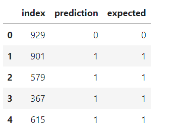
results = pd.DataFrame({'index':col1, 'prediction':col2, 'expected':col3})
results.head()
Creating Predictions on the Test Set
# Generate predictions with the best methodology
clf = AdaBoostClassifier()
clf.fit(X, y)
dfTestPredictions = clf.predict(X_test1)
# Write predictions to csv file
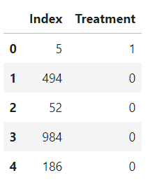
results = pd.DataFrame({'Index': X_test1.index, 'Treatment': dfTestPredictions})
# Save to file
results.to_csv('results.csv', index=False)
results.head()
Submission
results = pd.DataFrame({'Index': X_test1.index, 'Treatment': dfTestPredictions})
results
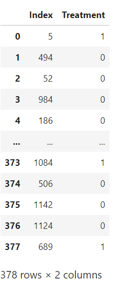
The final prediction consists of 0 and 1. 0 means the person is not needed any mental health treatment and 1 means the person is needed mental health treatment.
Conclusion
After using all these Employee records, we are able to build various machine learning models. From all the models, ADA–Boost achieved 81.75% accuracy with an AUC of 0.8185 along with that we were able to draw some insights from the data via data analysis and visualization.
The media shown in this article is not owned by Analytics Vidhya and is used at the Author’s discretion.


