This article was published as a part of the Data Science Blogathon.
Introduction
Customer Churn Prediction is one of the most enlightened problem statements nowadays as possibly everything is done to make a profit from business and that profit comes from customers that the company holds from its products and services so the goal of the organization is to hold up their permanent customers and analyze the potential one who may choose other alternatives this condition is known as the customer churn.
In this blog, we will build the potential model to predict customer churn with the help of PySpark’s MLIB library.

Problem Statement for Customer Churn Prediction
Let’s not take it as just an article from now on let’s suppose that we are working for a marketing agency who has hired us to draw a prediction about the potential customers who might stop buying their marketing services i.e customer churn.
Approach towards Customer Churn Prediction
As we are working on a real-world project so let’s understand the flow of it. Firstly one important thing to mention is that we have the “new_customer” independent data which will eventually be used as the testing data after the model development phase. We also need to create a classification algorithm that would help to classify based on the features we fed to the model whether customers will churn or not.
About the Dataset
This is the data of the marketing agency which has altogether 8 features and 1 target variable. If you want to know more about this dataset then go through this link.
- Name: Name of the company whom the customer is tagged to
- Age: Age of the Customer
- Total_Purchase: Total Ads Purchased
- Account_Manager: Binary 0=No manager, 1= Account manager assigned
- Years: Total Years of customers using the company service
- Num_sites: Total number of websites that are using this service.
- Onboard_date: Onboarding date of the latest contacted person.
- Location: Head Quarter address of the client
- Company: Name of Client’s Company
Importing Libraries and Starting the Spark Session
Here we are starting the first phase where the required libraries are imported for setting up the Spark environment and starting the Spark Session which is always the mandatory step to get started with PySpark.
from pyspark.sql import SparkSession

spark = SparkSession.builder.appName('customer_churn_prediction').getOrCreate()
spark
Output:
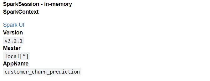
Inference: In the first step Spark Session module is imported with the pyspark.sql library and then for building and creating the SparkSession builder and getOrCreate() methods are used respectively.
Note that when we are looking at the GUI version of the session then we can see the App name, Version of the Spark, and the location where the session is created.
Reading the Dataset
In this section, we will be reading our dataset which includes all the features that are required to predict which customer is most likely to be churned and think of other alternatives.
data = spark.read.csv('customer_churn.csv',inferSchema=True,
                     header=True)
Inference: In the above line of code we have read the CSV formatted data using the read.csv function and put the inferSchema and header parameter as True so that we can see the real essence of the dataset.
data.printSchema()
Output:
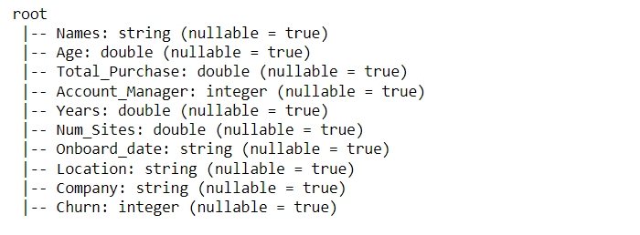
Inference: Printing the Schema of the data is one of the best practices to know about the type of each column like what kind of data it can hold. From the above output, it is shown that Onboard_date is of String type so in the following code if this feature is required then we should convert it to proper date format (if needed)
Let’s do some statistical analysis of our dataset where describe method alone can provide lots of insights into the statistics of the dataset.
data.describe().show()
Output:

Inference: The very first inference that we can draw is there are no NULL values in the dataset as the count is 900 for all the features hence we got rid of dealing with missing values. Then after looking at the mean and standard deviation of the Names column we can conclude string type doesn’t contribute anything to statistical analysis.
data.columns
Output:
['Names',
 'Age',
 'Total_Purchase',
 'Account_Manager',
 'Years',
 'Num_Sites',
 'Onboard_date',
 'Location',
 'Company',
 'Churn']
Inference: The column object is used only to get the names of all the columns that the current instance of the dataset’s variable holds and in the above output one can see the same.
Feature Selection
As we all are well aware feature selection is one of the most important steps in data preprocessing where we select all the features that based on our knowledge would be the best fit for the model development phase. Hence here all the valid numerical columns will be taken into account.
from pyspark.ml.feature import VectorAssembler

assembler = VectorAssembler(inputCols=['Age',
 'Total_Purchase',
 'Account_Manager',
 'Years',
 'Num_Sites'],outputCol='features')
Inference: While working with MLIB we should know the format of data that MLIB as a library accepts hence we use the VectorAssembler module which clubs all the selected features together in one column and that is treated as the feature column (summation of all the features), the same thing we can see in the parameter section of the assembler object.
output = assembler.transform(data)
Inference: Transforming the data is very much necessary as it works as the commit statement i.e. all the transactions (changes) which are processed should be seen in the real dataset if we see it hence we used the transform method for it.
final_data = output.select('features','churn').show()
Output:
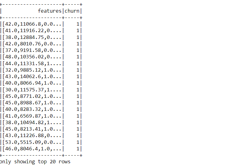
Inference: So while looking at the above output things will get clear that what we were aiming to do as the first column is features that have all the selected columns and then the label column i.e. churn.
Test Train Split
Now if you are following me from the very beginning of the article might have a question if we already have the separate testing data then why are splitting this dataset? right?
So the answer is to keep this phase of splitting as the validation of the model and we do not have to perform this routine again when we would be dealing with new data as it is already split into different CSV files.
train_churn,test_churn = final_data.randomSplit([0.7,0.3])
Inference: With the help of tuple unpacking we have stored the 70% of the data in train_churn and 30% of it in test_churn by using PySpark’s random split() method.
Model Development
We reaching this phase of the article is the proof that we have already cleaned our data completely and that it is ready to be fed to the classification algorithm model (more specifically the Logistic Regression)
Note that we have to do this model building again when we have to deal with new customers’ data.
from pyspark.ml.classification import LogisticRegression
lr_churn = LogisticRegression(labelCol='churn')
fitted_churn_model = lr_churn.fit(train_churn)
training_sum = fitted_churn_model.summary
Code breakdown: This would be a complete explanation of the steps that are required in the model building phase using MLIB
- Importing the LogisticRegression module from the ml. classification library of the Pyspark.
- Creating a Logistic Regression object and passing the label column (churn).
- Fitting the model i.e. starting the training of the model on the training dataset.
- Getting the summary of the training using the summary object which was attained over the trained model
training_sum.predictions.describe().show()
Output:

Inference: So the summary object of the MLIB library returned a lot of insights about the trained logistic regression model and with the statistical information available we can conclude that model has performed well as the mean, standard deviation of the churn (actual values) and prediction (predicted values) is very close.
Model Evaluation
In this stage of the customer churn prediction, we should analyze our model which was trained on 70% of the dataset and by evaluating it we can decide whether we should go with the model or if some twitches are required.
from pyspark.ml.evaluation import BinaryClassificationEvaluator
pred_and_labels = fitted_churn_model.evaluate(test_churn)
Inference: One can notice that in the first step we imported the BinaryClassificationEvaluator which is quite logical as well because we are dealing with the label column that has binary values only.
Then evaluate() method comes into existence where it takes the testing data (30% of the total dataset) as the parameter and returns the multiple fields from which we can evaluate the model (manually).
pred_and_labels.predictions.show()
Output:
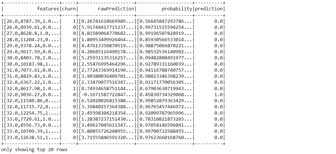
Inference: In the above output one can see 4 columns that were returned by the evaluation method they are:
- Features: All the feature values were clubbed together by VectorAssembler during the feature selection phase.
- Customer Churn: The Actual values i.e. the actual label column
- Probability: This column have the probability of the predictions that were made by the model.
- Predictions: The predicted values (here 0 or 1) by the model on the testing data.
Predicting the New Data
Finally comes the last stage of the article where till now we have already built and evaluated our model and now here the predictions will be made on the completely new data i.e. the new customer’s dataset and see how well the model performed.
Note that in this stage the steps will be the same but the dataset will be different according to the situation.
final_lr_model = lr_churn.fit(final_data)
Inference: Yes! Yes! nothing extra to discuss here as we have already gone through this step but the main thing to notice is that we are performing the training on the complete dataset (final_data) as we know we already have the testing data in the CSV file hence no splitting of the dataset is required.
new_customers = spark.read.csv('new_customers.csv',inferSchema=True,
                              header=True)

new_customers.printSchema()
Output:

Inference: As the testing data is in a different file then it becomes necessary to read it in the same way we did it before in the case of the customer_churn dataset.
Then we saw the Schema of this new dataset and concludes that it has the exactly same Schema.
test_new_customers = assembler.transform(new_customers)
Inference: Assembler object was already created while the main features were selected so now the same assembler object is being used to transform this new testing data.
final_results = final_lr_model.transform(test_new_customers)
Inference: As we did the transformation of the features using assembler object similarly we also need to do the transformation of the final model on top of new customers.
final_results.select('Company','prediction').show()
Output:
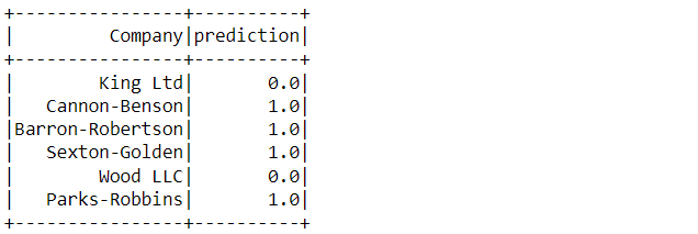
Inference: Here comes the data which we were aiming to achieve where we could know that the companies like Cannon-Benson, Barron-Robertson, Sexton-GOlden, and Parks-Robbins need to assign an Account Manager to decrease the churn of the customers.
Conclusion to Customer Churn Prediction
This is an important aspect of the article where I’ll try to give a brief about everything we did in this article like how we can assign the Account Managers to the customers to decrease the rate of churn in those particular companies and discuss each step in brief.
- First, we read the customer churn data and analyzed it both statistically and logically.
- Then we selected the main features that could be the best fit for the model development phase after splitting the dataset (for this instance it was required)
- Then after building the model we evaluated it too using the BinaryClassificationEvaluator which helped us to know how well our model performed on testing data.
- Then we did the same process on top of the new dataset (new testing data) i.e. feature selection, model building, and at the last making predictions that in the end helped in knowing which company requires the Account Manager.
The media shown in this article is not owned by Analytics Vidhya and is used at the Author’s discretion.


