This article was published as a part of the Data Science Blogathon.
Introduction
The structured data we generally deal with gets stored in a tabular format in relational databases. And stored data in these databases can be accessed by a query language called “sequel” or SQL. And it is a powerful language. But, it is a pain to write raw SQL codes when dozens of databases use a different flavor of SQL; it becomes even tougher to migrate to other databases as their syntaxes vary. But what if there’s a tool that masks all these complications and lets us write pure Pythonic code to communicate with backend databases? Well, this is where SQL Alchemy comes into the picture.

So, in this article, we will discuss how we can leverage the power of SQL Alchemy to interact with backend databases without writing any SQL code directly. But before that, we’re going to get acquainted with SQL Alchemy.
Table of contents
What is SQL Alchemy
So, SQL Alchemy is a database toolkit written in Python for Python. The API consists mainly of two distinct parts, one is the Alchemy core, and the other is Alchemy ORM. The ORM is built on top of the Alchemy core. Hence, most operations of the core are also applicable to the ORM. So, what are these cores and ORMs?
Alchemy Core forms the basis of the toolkit. The core provides an abstraction layer on different DBAPI implementations and behaviors. The SQLAlchemy Expression Language presents a system of representing relational database structures and expressions using Python constructs
The other part of SQLAlchemy is its ORM or Object Relationship Mapper. The object-relational mapping is the concept of writing complicated SQL queries using an object-oriented paradigm. So, indeed, we intend to write SQL queries in our preferred language. The Alchemy ORM is an applied use case of alchemy expression language.
In this article, we will shed some light on the expression language.
Installing Requirements
Before we go into the coding part, we need to install requirements. First, install the SQL Alchemy library itself. A simple pip statement should be enough for this.
pip install sqlalchemyNext up, we will need to install the DBAPI of our backend database dialect. SQL has many dialects like any human language. For example, Mandarin and Cantonese are dialects of the Chinese language. Usually, the RDBMS provided by different organisations may slightly differ in terms of syntaxes. Oracle, MySQL, SQLite, PostgreSQL, and MS SQL are called SQL dialects. So, as per the database you use, install the appropriate DBAPI. We will use SQLite for this article. Let’s see how to set it up.
First, we need to create an engine to specify DBAPI.
import sqlalchemy as sa
engine = sa.create_engine('sqlite:///D:/baseball.db') #Create baseball.sqlite
SQLite deals with the local files, so the URLdiffers from other dialects.
Let’s see how we can create an engine for the MySQL dialect.
engine = sa.create_engine('mysql+mysqldb://root:password@localhost/database name')In the above code, the first part mentions the dialect and DBAPI double slash followed by the username, password, server name and at the end, the name of the database. The rest of the dialects follow the same pattern mentioned above. Just make sure to download compatible DBAPI for your database. It assumes the default API for that backend is available in the system if you haven’t mentioned the DBAPI. Below is the code snippet for making a connection to a database.
engine = sa.create_engine('sqlite:///D:/student.db')
connection = engine.connect()
We still haven’t established a connection to the database yet. An actual connection to the database is made when we supply a query to the database. Another important thing is that I don’t have any database named student in my system. So, if you pass in a database name along with its path, SQLite will create a brand new database in that location.
Creating a Table
Now, we will see how we can create a database and tables with the help of SQL Alchemy. We will create a simple table named students with ID as the primary key and two string-type columns and addresses.
from sqlalchemy import Table, Column, Integer, String, MetaData, ForeignKey
metadata_obj = MetaData()
users = Table('student', metadata_obj,
    Column('id', Integer, primary_key=True),
    Column('name', String),
    Column('address', String),
)
The metadata object stores the schema details of the table. Let’s now insert a row in the table.
ins = users.insert().values(name='Rakesh', address='Bhubaneswar')
result = connection.execute(ins)
We can similarly insert multiple rows to the table as well.
ins = users.insert()
connection.execute(ins, [{"id": 2, "name":"Sonu", "address": "Chennai"},
                        {"id": 3, "name":"Dibya", "address": "Kurukshetra"},
                        {"id": 4, "name":"Rahul", "address": "Indore"}])
Let’s see it in our data table.
query = sa.select([users])
Result = connection.execute(query)
ResultSet = Result.fetchall()
print(ResultSet[:])
Output: [(1, 'Rakesh', 'Bhubaneswar'), (2, 'Sonu', 'Chennai'), (3, 'Dibya', 'Kurukshetra'), (4, 'Rahul', 'Indore')]
Update and Delete
Update and Delete are DML operations used to update and delete particular entries in the table that meet certain conditions.
Update
query = sa.update(users).values(adress = 'Bengaluru').where(users.c.name == 'Rakesh)
res = conn.execute(query)
query2 = sa.select([users])
res = conn.execute(query2)
res.fetchall()
Delete
query = sa.delete(users).where( users.c.id == 1)
res = conn.execute(query)
query2 = sa.select([users])
res = conn.execute(query2)
Querying From Table
Let’s see how we can perform regular SQL queries in Alchemy. For this, we will use a different database.
e
ngine = sa.create_engine('sqlite:///D:/baseball.db', echo = False)
connection = engine.connect()
metadata = sa.MetaData()
baseball = sa.Table('allstarfull', metadata, autoload=True, autoload_with=engine)
Columns of the table
baseball.columns.keys()output: ['index', 'playerID', 'yearID', 'gameNum', 'gameID', 'teamID', 'lgID', 'GP', 'startingPos']
Let’s see how the data table looks like
query = sa.select([baseball])
result = connection.execute(query)
result.fetchmany(5)
output:[(0, 'gomezle01', 1933, 0, 'ALS193307060', 'NYA', 'AL', 1.0, 1.0),
 (1, 'ferreri01', 1933, 0, 'ALS193307060', 'BOS', 'AL', 1.0, 2.0),
 (2, 'gehrilo01', 1933, 0, 'ALS193307060', 'NYA', 'AL', 1.0, 3.0),
 (3, 'gehrich01', 1933, 0, 'ALS193307060', 'DET', 'AL', 1.0, 4.0),
 (4, 'dykesji01', 1933, 0, 'ALS193307060', 'CHA', 'AL', 1.0, 5.0)]
To make the table look better and more understandable, we can convert it to a data frame
import pandas as pd
df = pd.DataFrame(result.fetchmany(5), columns=result.keys())
print(df)

**fetchmany() and fetchall() are the functions used to retrieve a specific number of elements from the table. We can limit the number of imported rows by passing an argument in fetchmany(n).
Where Clause
We will query details of the first four players having team ID NYA (New York Yankees) and year ID after 2000.
query = sa.select([baseball]).where(sa.and_((baseball.columns.teamID=='NYA'), baseball.columns.yearID>2000))

result = connection.execute(query)

df = pd.DataFrame(result.fetchmany(5), columns=result.keys())

df

Order By and Group By
Group By and Order By are two necessary SQL commands. Let’s see how we can perform these operations using Alchemy.
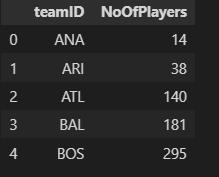
query = sa.select( baseball.c.teamID, sa.func.count(baseball.c.playerID).label('NoOfPlayers'))
                                                                    .group_by(baseball.c.teamID)
result = connection.execute(query)
df = pd.DataFrame(result.fetchmany(5), columns=result.keys())
df

As you can observe, we used an aggregate function along with GROUP BY. The label function works just as “AS” in SQL to specify the alias of a column. Similarly, we can also use order by command.
query = sa.select( baseball.c.teamID, sa.func.count(baseball.c.playerID).label('NoOfPlayers'))
                                                                    .group_by(baseball.c.teamID)
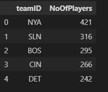
                                                                    .order_by(sa.desc('NoOfPlayers'))
result = connection.execute(query)
df = pd.DataFrame(result.fetchmany(5), columns=result.keys())
df

In the above code, Order by was used with the descending function on the alias of the aggregated column.
SQL Join
Usually, we have to work with multiple tables, and to query data from them requires joining. We will be using an inner join method.
For this, we will use two separate tables from Chinook data.
engine = sa.create_engine('sqlite:///E:/Chinook.sqlite', echo = False)
conn = engine.connect()
metadata = sa.MetaData()
artist = sa.Table('Artist', metadata, autoload=True, autoload_with=engine)
album = sa.Table('Album', metadata, autoload=True, autoload_with=engine)
The artist table has the name of the artists and their IDs. While the album table has artist IDs, the name of the album, and their IDs. So, we will be joining these two tables on the Artist Id column.
query = sa.select([album, artist.c.Name])
j = album.join(artist, album.c.ArtistId == artist.c.ArtistId )
stmt = query.select_from(j)
res = conn.execute(stmt)
dt = pd.DataFrame(res.fetchmany(5), columns=res.keys())
dt

The SQL equivalent of the above code is
str(stmt) output: ‘SELECT “Album”.”AlbumId”, “Album”.”Title”, “Album”.”ArtistId”, “Artist”.”Name” nFROM “Album” JOIN “Artist” ON “Album”.”ArtistId” = “Artist”.”ArtistId”‘Pros and Cons of SQL Alchemy
Now, let’s discuss some advantages and drawbacks of SQL Alchemy.
Pros
- Alchemy gives abstraction to the backend database. So, an average developer does not have to worry about SQL statements.
- The transition to other databases becomes easier.
- Queries are optimized and may work better than SQL if you wrote it yourself unless you are an SQL veteran.
Cons
- There could be instances where Alchemy might become inefficient. Therefore, knowing SQL is always desired.
- Knowing what is happening under the hood often gives an edge. So, it is not a complete replacement for SQL.
Applying the SQLAlchemy API
SQLAlchemy is a Python library that makes it easier to work with databases. It allows you to create objects representing your data and then use them to interact with the database. This can make your code more readable and maintainable, and it can also help you to avoid errors.
Here are some of the key things that SQLAlchemy can do for you:
- Create and manage database tables
- Insert, update, and delete data from tables
- Run complex queries on your data
- Manage transactions to ensure that your data is consistent
If you are working with databases in Python, then SQLAlchemy is a valuable tool that can make your life easier.
Conclusion
Throughout the article, we went through different concepts regarding SQL Alchemy. We learned the What and Why of Alchemy. In this article, we grazed the surface of expression language. Few key points from our article
- First, we learned how to connect to databases in different SQL dialects.
- We learned to create a new table from scratch and import existing tables.
- Learned to use basic SQL operations like querying, Aggregating, joining, Updating and Deleting, etc.
- Finally discussed the pros and cons of Alchemy in brief.
So, this was it. Thank you for reading.
Frequently Asked Questions
SQLAlchemy supports databases such as MySQL, PostgreSQL, SQLite, and more.
SQLAlchemy is a versatile tool that works with various databases, including SQLite. On the other hand, SQLite is a specific type of database. Think of SQLAlchemy as a toolbox with many tools, and SQLite is one of those tools.
SQLAlchemy provides flexibility to work with different databases, simplifies complex queries, and offers an easy-to-use ORM (Object-Relational Mapping) for interacting with databases in a Pythonic way. It makes handling databases more straightforward and efficient.
The media shown in this article is not owned by Analytics Vidhya and is used at the Author’s discretion.


