This article was published as a part of the Data Science Blogathon.
Introduction to Intelligent Search Algorithms

Search problems are widespread in real-world applications. Search algorithms are beneficial in simplifying or solving the problems such as searching a database or the internet. One of the most popular search problems is to find the shortest path between two nodes on a grid. Many interesting applications similar to Google Maps use Intelligent search algorithms to execute requests to find the most optimal path between two cities or places. In this article, we discuss all the foundational to state-of-art algorithms used in applications like Google Maps to solve search problems similar to finding the shortest path. We start with defining the problem of finding the shortest path between two nodes in a grid. Then we discuss algorithms that are foundational to the most powerful and smart search A* algorithm, (Depth First Search) DFS, (Breadth First Search) BFS, and Greedy Best First Search (GBFS). We try to understand the complete A* algorithms, one of the most powerful and smart algorithms among search problems while covering the overview of fundamental algorithms. Finally, we wrap up the article by discussing some key ideas that enable A* to be the most optimal search algorithm for finding the shortest path and discuss the variations of A* algorithms.
Note: In these algorithms, a subset of search algorithms is related to finding the shortest path. Search algorithms are used to build AI game players that play games like tic-tac-toe or chess by using adversarial algorithms (which can be covered in the upcoming article).
Definition
Finding the shortest distance or path between two grid nodes is a widespread search problem. Efficient algorithms for finding the shortest path are embedded in services like Google maps to estimate the optimal path upon users’ input. An informal definition of the problem statement is, given two nodes/cells A and B in a grid/map, find the shortest optimal path from A to B.
Intelligent Search Algorithms
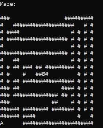
To find the shortest path between two cells on the grid (figure below), some fundamental search algorithms are classified into two kinds: informed and uninformed. Uninformed algorithms don’t utilise the information in the problem statement, similar to DFS (Depth First Search) and BFS (Breadth First Search); however, DFS doesn’t guarantee any optimal solution. Informed algorithms utilise the information in the problem statement to solve the problem more optimally in terms of computing cost or time, similar to Greedy Best First Search (GBFS) and A* algorithm. One of the very efficient algorithms, most popularly used to find the shortest between two cells or places on a map, is the A* algorithm.

Note: Throughout this article and in the code, the map or grid nodes are of a custom-defined class type with some properties, which are also defined in the code. Node is exclusively defined as a class that enables faster manipulation and implementation of informed algorithms GBFS and A*.
DFS (Depth First Search)
Depth First Search (DFS) is a graph traversal algorithm used to traverse through a graph in a depth-first fashion. In other words, the depth-first search algorithm explores a specific node to the complete depth until it reaches a dead end, only when it returns and explores another path available. DFS is often implemented using a first-in-last-out stack. The algorithm of DFS is described below:
1. Start with some arbitrary node, and push the node to an empty stack.
2. In a while loop, pop a node from the stack.
3. Expand the node, push the neighbours into the stack and explore through a specific node until it reaches a dead end.
4. Once it reaches a dead end, pop the top node in the stack and start exploring the node.
5. In this traversal, we find the solution if we find a goal or target. Otherwise, we conclude no solution possible.
Note: DFS guarantees no solution or optimal solution; hence, it is less often used in search problems like this.

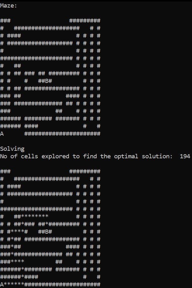
The above figure shows the output of the DFS algorithm on the maze mentioned earlier; the count defines the no of explored cells explored by DFS to reach the target. In this case, the no of explored states is 194. However, DFS doesn’t guarantee a solution.
The code illustrates the DFS algorithm here.
BFS (Breadth First Search)
An efficient alternative to DFS that guarantees an accurate solution but a non-optimal one is BFS. BFS uses a first-in-first-out queue data structure to traverse through the graph of nodes. The following algorithm describes the implementation details:
1. Start with an arbitrary node, and push the node to an empty queue.
2. In a while loop, pop a node from the queue.
3. Expand the node, push the neighbours into a queue and explore through a specific node till the end.
4. Once it reaches a dead end, pop the top node in the queue and start expanding and exploring that node.
5. In this traversal, we find the solution if we encounter a goal or target. Otherwise, no solution is found.

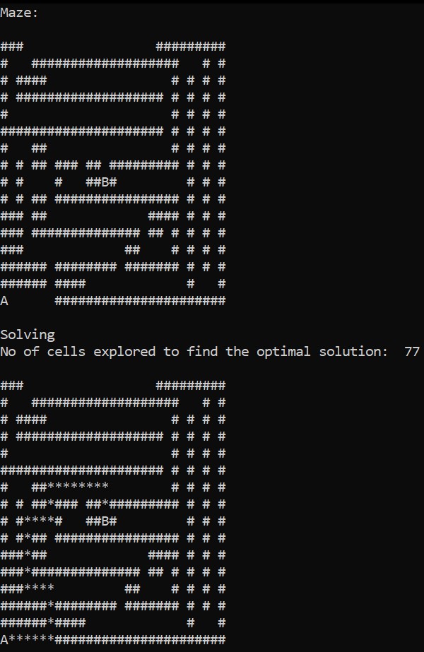
The figure above shows the output of the BFS algorithm on the maze mentioned before; the count defines the no of explored cells explored by DFS to reach the target. In this case, 77 is better than DFS. It is not guaranteed that BFS is more efficient than DFS, but BFS guarantees an accurate solution always, unlike DFS
The code illustrates the BFS algorithm here.
Greedy Best First Search (GBFS)
GBFS is an extension to BFS, which additionally uses the information in the problem statement to efficiently make decisions on the path chosen. GBFS associates a cost for each node on the grid, determining how far the current node is from the goal state. The cost associated with a node can be calculated in many ways; some of the commonly used distance heuristics are [2]:
1. Euclidean Distance
Euclidean distance is commonly used to make a choice of the path if in case the sample space is any direction.
cost = sqrt ((curr_node.x – target.x) ^2 + (curr_node.y – target.y) ^2 )
2. Manhattan Distance
Manhattan distance is commonly used to make a choice of path in either of the four orthogonal directions (like an elephant on a chess board).
cost = abs (curr_node.x – target.x) + abs (curr_node.y – target.y)
In the coding example, we consider Manhattan distance as a heuristic and proceed to select the nodes with the lowest estimated cost using the heuristics. The GBFS follows the same steps as BFS, except that it picks up a cost-efficient node, unlike BFS, which picks up a node on the top of the queue.

The figure above shows the output of the GBFS algorithm on the maze mentioned before; the count defines the no of explored cells explored by DFS to reach the target. In this case, 77, this case is same as BFS, but the extra potential of GBFS is that it is more significant in higher complex maze problems.
The below code linked here explains the GBFS algorithm for finding the shortest path using an informed algorithm.
A* algorithm
A* algorithm is a heuristic-based search algorithm developed from the greedy best-first search in which the algorithm uses the data of the position of the target cell to carefully make the choice of paths. A* on a better version of GBFS uses an extra heuristic function to make the choice of paths.
A* uses two heuristics to efficiently decide the choice of path, one is to calculate the distance from the current cell to a target like GBFS, and the other is to keep track of the distance travelled from the start cell to the current cell. Using the two heuristics unleashes the power to choose a better choice among the possible paths since the first heuristic guides to choose a closer path. In contrast, the second heuristic ensures the current path is short and doesn’t lead to paths like round-about or internal curves. In this way, the two heuristics finally lead the algorithm to not only find the solution but with an optimized cost approach.

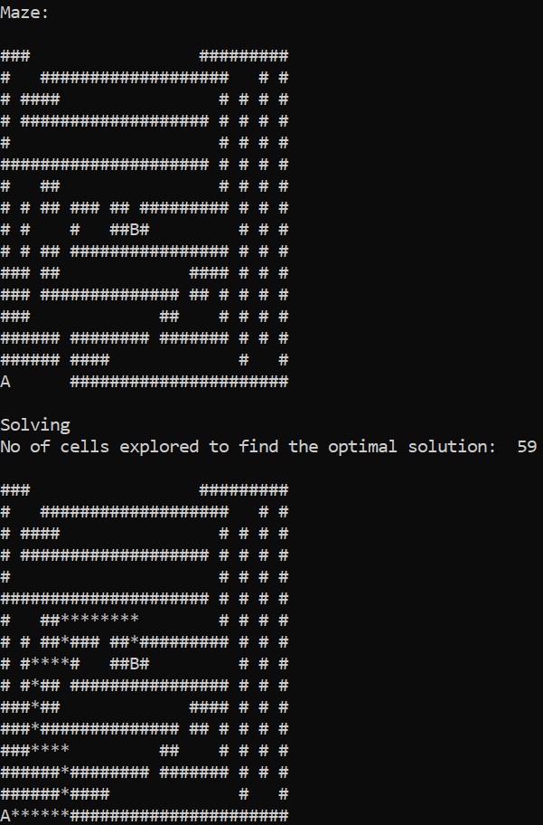
The figure above shows the output of the A* algorithm on the maze mentioned before; the count defines the no of explored cells explored by DFS to reach the target. In this case, 59 is better than GBFS.
The code is linked here, explaining the A* algorithm with implementation.
From the no of steps the GBFS and A* explored to reach the target state, we can conclude that the A* algorithm guarantees an optimal path by making efficient guesses using heuristics.
Conclusion to Intelligent Search Algorithms
In this article, we have taken an exhaustive tour of the foundational intelligent search algorithms, especially for finding the shortest optimal path between two nodes, one of the most common search problems, and implementing them.
1. Firstly, we started by defining the problem of finding the shortest path and classified the types of algorithms, informed & uninformed.
2. We have briefed on the uninformed algorithms such as DFS and BFS, including their performance in multiple scenarios.
3. We discussed the more complex search algorithms like GBFS and the A* algorithm.
4. Moreover, we have understood through a brief understanding of different distance heuristics used in A* and GBFS, or more generally, in informed algorithms.
5. Finally, we compared the performances and conclude the efficacy of informed algorithms, especially the A* algorithm.
I hope you enjoyed reading my article on intelligent search algorithms. If there is some feedback, then please share it in the comments section below.
The media shown in this article is not owned by Analytics Vidhya and is used at the Author’s discretion.


