Introduction
One of the most important applications of Statistics is looking into how two or more variables relate. Hypothesis testing is used to look if there is any significant relationship, and we report it using a p-value. Measuring the strength of that relationship is as important, if not more and effect size is the number used to represent that strength.[1]
For example, in addition to looking into whether the new medicine is better than the old one using a p-value, we should also measure how much better the new medicine is using effect size.
In machine learning problems, the effect size can also be used in feature selection.
We can categorize effect sizes based on the type of variables involved (e.g., Categorical or Non-Categorical).
Let’s look into different types of effect sizes and calculate them using various Python libraries.
Continuous-Continuous Variables- Python Function
When data is parametric(i.e., data is normally distributed and correlation is linear), we can use Pearson correlation.
Pearson correlation coefficient
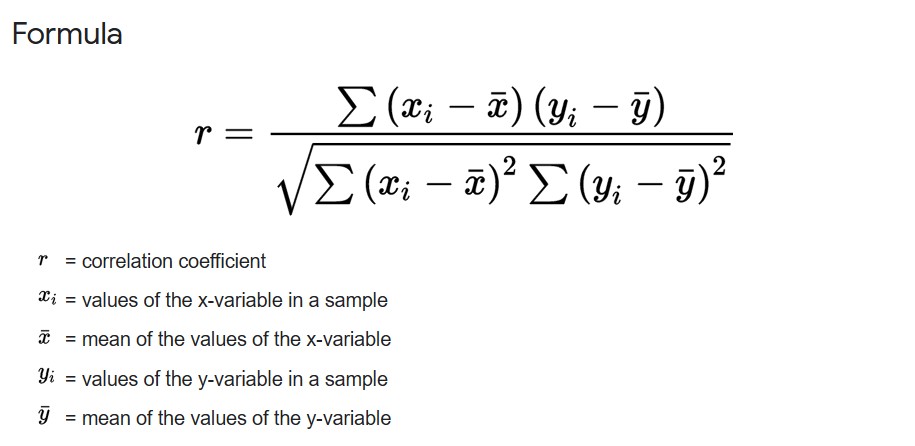
For Correlation between two continuous variables, we measure how the value of each variable at ith index changes w.r.t. to the variable’s mean.
 pearson r
Pearson’s r has a range between -1 and 1. A value closer to 0 indicates a weak correlation, and a value closer to -1 or 1 indicates a strong negative or positive correlation.
Correlation using NumPy library for variables x and y.
import numpy as np

np.corrcoef(x, y)
The above function returns the correlation coefficient matrix of variables.
If the data is in the panda’s data frame(df), the following function can be used for the correlation coefficient matrix of numerical variables.
import pandas as pd

df.corr()
Spearman’s rank correlation coefficient
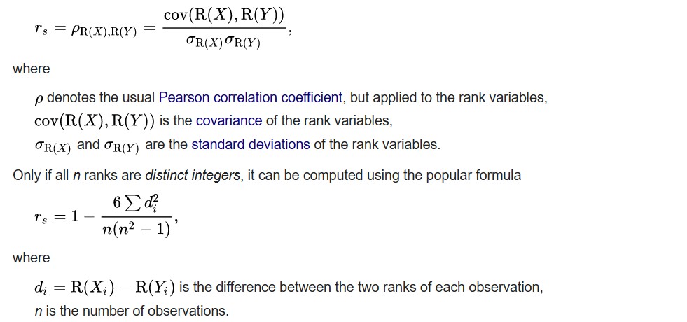
When data is non-parametric, Spearman’s correlation coefficient can be used. Rather than comparing the values, we compare the ranks of values of each variable at ith index.
The formula for Spearman’s r.

Python function to calculate Spearman’s rho using scipy:
from scipy import stats
print(stats.spearmanr([1,2,3,4,5], [5,6,7,8,7])) # this will output correlation and p-value
Using Pandas
df.corr(method='spearman')
Categorical-Continuous Variables – Python Function
When one variable is categorical and another is non-categorical, we can determine how much statistical dispersion across all values can be explained by dispersion among the categories.
The correlation ratio (eta) can be used to see if one or more categories have more influence among all categories.
First, we calculate the mean value of each category and the mean of all values.

where
y
¯
x
{displaystyle {overline {y}}_{x}} is the mean of the category x and
y
¯
{displaystyle {overline {y}}} is the mean of the whole population.
Then, we calculate the ratio of the weighted sum of the squares of the differences between each category’s average and overall average to the sum of squares between each value and overall average.
correlation ratio(eta)

Calculation of correlation ratio (eta) in Python.
import numpy as np
import pandas as pd

def correlation_ratio(categories, measurements):
    fcat, _ = pd.factorize(categories)
    cat_num = np.max(fcat)+1
    y_avg_array = np.zeros(cat_num)
    n_array = np.zeros(cat_num)
    for i in range(0,cat_num):
        cat_measures = measurements[np.argwhere(fcat == i).flatten()]
        n_array[i] = len(cat_measures)
        y_avg_array[i] = np.average(cat_measures)
    y_total_avg = np.sum(np.multiply(y_avg_array,n_array))/np.sum(n_array)
    numerator = np.sum(np.multiply(n_array,np.power(np.subtract(y_avg_array,y_total_avg),2)))
    denominator = np.sum(np.power(np.subtract(measurements,y_total_avg),2))
    if numerator == 0:
        eta = 0.0
    else:
        eta = np.sqrt(numerator/denominator)
    return eta
The range of eta is between 0 and 1. A value closer to 0 indicates all
categories have similar values, and any single category doesn’t have more
influence on variable y. A value closer to 1 indicates one or more
categories have different values than other categories and have more influence on variable y.
Eta can be used in EDA and data processing to know which categorical features are more important in machine learning model building.
The function can calculate eta for various columns in a data frame.
def cat_cont(df, categorical_features, continuous_features):
    eta_corr = []
    for pair in itertools.product(categorical_features, continuous_features):
        try:
            eta_corr.append(correlation_ratio(df[pair[0]], df[pair[1]]))
        except ValueError:
            eta_corr.append(0)
    eta_corr = np.array(eta_corr).reshape(len(categorical_features),len(continuous_features))
    eta_corr = pd.DataFrame(eta_corr, index=categorical_features, columns=continuous_features)
    return eta_corr
Here, categorical_features and continuous features list categorical and continuous columns in data frame df.
Once we have the eta value, we can compare any two categories to look into the difference between the values of each category.
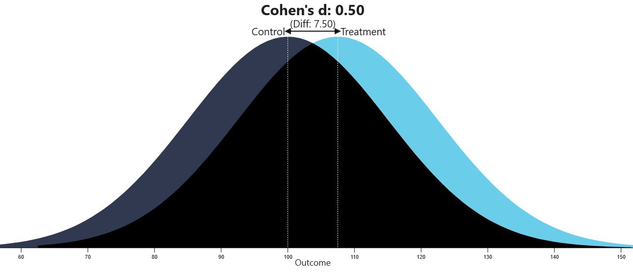
Cohen’s d
Cohen’s d can be used to calculate the standardized difference between two categories.
Here’s the Python function to calculate Cohen’s d value.
import numpy as np

def cohend(d1, d2):
    # calculate the size of samples
    n1, n2 = len(d1), len(d2)
    # calculate the variance of the samples
    s1, s2 = np.var(d1, ddof=1), np.var(d2, ddof=1)
    # calculate the pooled standard deviation
    s = np.sqrt(((n1 - 1) * s1 + (n2 - 1) * s2) / (n1 + n2 - 2))
    # calculate the means of the samples
    u1, u2 = np.mean(d1), np.mean(d2)
    # calculate the effect size
    return (u1 - u2) / s
The value of Cohen’s d varies from 0 to infinity.
The below-mentioned website can be used to visualize different Cohen’s d values.
Visualization of Cohen’s d (from https://rpsychologist.com/cohend)

Source: https://rpsychologist.com/cohend/
Categorical-Categorical Variables- Python Function
Cramer’s V can be used for correlation between two categorical variables based on the chi2 test statistic.
Here’s the python function to calculate Cramer’s V.
import scipy
def cramers_v(x, y):
    confusion_matrix = pd.crosstab(x,y)
    chi2 = scipy.stats.chi2_contingency(confusion_matrix)[0]
    n = confusion_matrix.sum().sum()
    phi2 = chi2/n
    r,k = confusion_matrix.shape
    phi2corr = max(0, phi2-((k-1)*(r-1))/(n-1))
    rcorr = r-((r-1)**2)/(n-1)
    kcorr = k-((k-1)**2)/(n-1)
    return np.sqrt(phi2corr/min((kcorr-1),(rcorr-1)))
The following function can find Cramer’s V in a data frame with categorical variables.
def cat_cat(df, cat_features):
    cramers_v_corr = []
    for pair in itertools.product(cat_features, repeat=2):
        try:
            cramers_v_corr.append(cramers_v(df[pair[0]], df[pair[1]]))
        except ValueError:
            cramers_v_corr.append(0)
    cramers_v_corr = np.array(cramers_v_corr).reshape(len(cat_features),len(cat_features))
    cramers_v_corr = pd.DataFrame(cramers_v_corr, index=cat_features, columns=cat_features)
    return cramers_v_corr
Here cat_features is a list of categorical columns in data frame df.
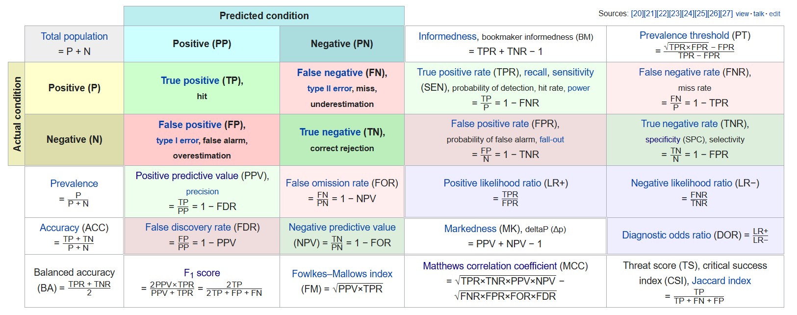
Another common way to describe associations among two or more categorical variables is the Confusion Matrix.
Various metrics related to the confusion matrix are as follows

Precision or specificity can be used among the various metrics available if we want to measure false positives.
Similarly, recall(same as sensitivity) can be used if we want to measure false negatives.
F1 score can be used to take into account both precision and recall. Since the f1 score is not considering true negatives, it’s useful only when the majority class is labeled as negative(i.e., negatives are a lot more than positives).
Otherwise, Matthews Correlation coefficient (MCC) can be used, similar to Cramer’s V.
A detailed article about the confusion matrix is published here.
Various correlations mentioned above can be directly calculated from this library – http://shakedzy.xyz/dython/
Conclusion
In this article, we have understood why effect size is important and its various applications.
Then, we learned about measuring effect sizes for different combinations of variables and their implementation in Python.
And we have created various functions to calculate correlations in a data frame having categorical and continuous columns.
We can list the following takeaways from the article.
- Effect size is important to measure, especially in machine learning problems.
- Different effect sizes can be calculated for combinations of categorical and continuous variables.
- We can calculate effect sizes for all data frame columns by making custom functions.


