This article was published as a part of the Data Science Blogathon.
Introduction
Data cleaning is one area in the Data Science life cycle that not even data analysts have to do. Still, data scientists and their daily task are to clean the data so that machine learning algorithms will have the data good enough to be fed. Hence we need to have some sort of template for cleaning the dataset.
In this article, we will learn how to clean a dataset, i.e., some mandatory steps required that one has to know before getting started with the data preparation phase of a data science project. In this way, the newbies who have started their journey will understand the critical steps in cleaning/preparing the dataset for different processes like feature engineering and machine learning model development.
In a nutshell, we will try to build a template for data cleaning using Python and its famous libraries (Numpy and Pandas).

The very first thing that we should do before actually getting started with data cleaning is – Ask Questions to ourselves i.e. What insights you wanna draw from your analysis? what needs to be corrected based on the business requirements? Similarly, we have curated down some of the key tasks for us (particularly for this instance):
- How does the dataset handle invalid values?
- What do we want to do with null values?
- Do we want to summarise, group, or filter the data?
Importing Libraries Required for Data Cleaning
Firstly, we will import all the libraries required to build up the template.
import pandas as pd2
import numpy as np
Pandas and Numpy are the most recommended and powerful libraries when it comes to dealing with structured data or the tabular data
- Pandas: Pandas are tagged as the data manipulation library by every data analyst (both experienced and freshers) as it is enriched with vital functionalities and more than everything to deal with tabular data.
- Numpy: Numpy is mainly used to work with arrays and complex mathematical calculations by providing some useful functions in linear algebra, Fourier transform, and matrices.
import pandas as pd
import numpy as np
df = pd.read_csv(“diabetes.csv”)
df.info()
Inference: Firstly we started with reading the dataset (this is the famous Diabetes dataset from the UCI machine learning repository) using the read.csv() function. Then for further intervention using the info() method, which is giving us the following insights:
- Does our dataset have any null values? The answer is no! as we can see 768 non-null values.
- Real data types are detected for each column for BMI and Pedigree function it is a float. For the rest, it is an integer.
df.head()
Output:

Inference: So it looks like they are using 0 values where they don’t have data. I don’t think they’re using NaN at all, but if they were we could either drop those rows (drop a) or fill them to some value (file). Because they’re using 0 already, it might be prudent to do this just in case.
df = df.fillna(0)
Inference: So now we know there are NaN values. We could also have just, you know, checked for NaN, but now I’m trying to show functions you can use.
So, what to do with these zero values? Sometimes, we could fill them with something sensible, but that normally just biases the data. So mostly, we’d ignore them. So we want to ask how we want to use the data. Will we be using SkinThickness? Do we care if there are non-physical outliers?
If we primarily cared about Glucose, BMI, and Age, we could get rid of a ton of these issues but only look at those columns.
df2 = df[["Glucose", "BMI", "Age", "Outcome"]]
df2.head()
Output:

Inference: Here, we have grabbed the columns in which we are more interested to do our analysis, and this can be a widespread and essential step in any data cleaning process as we don’t need all the columns in hand to deal with. Hence selecting the right set of data is very important.
One can notice that We chose the Glucose, BMI, Age, and Outcome column, where the last one is the target, and the rest are features. They are extracted using multi-indexing.
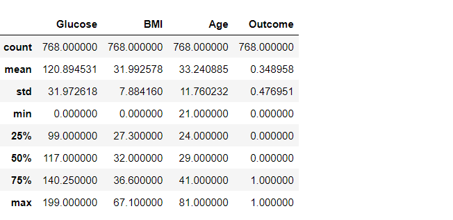
df2.describe()
Output:

Inference: But now, let’s get rid of any stray zeros. What we want to do is find a row with any number of zeros and remove that row. Or in terms of applying a mask, find the rows which have any zero (True), and invert that (to False) so when we apply the mask using loc, the False entries get dropped.
df3 = df2.loc[~(df2[df2.columns[:-1]] == 0).any(axis=1)]
df3.describe()
df3.info()
Output:

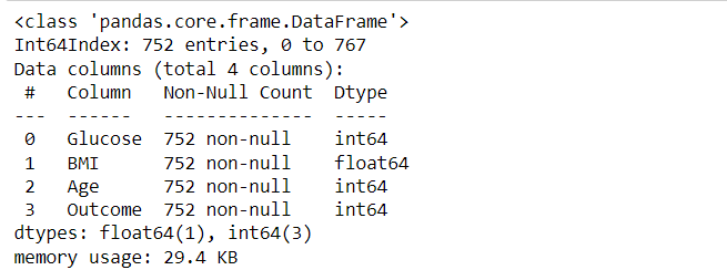
Inference: Great, so we’ve selected the data we cared about and ensured it has no null-like values. We’ll go on to check things look sane with some plots in the next section. One final thing we could do is to group the data by the outcome. It might make it easier to look for patterns in diagnoses.
We can do this either by splitting out the DataFrame into two (one for yes and one for no), or if we wanted summary statistics, we could use the groupBy function:
df3.groupby("Outcome").mean()
Output:

Inference: What this can tell us is that, in general, the higher your glucose level, the more overweight you are, and the older you are, the greater your chance of being diagnosed with diabetes. Which, perhaps, is not that surprising.
We can do other things using the group by the statement, like so:
df3.groupby("Outcome").agg({"Glucose": "mean", "BMI": "median", "Age": "sum"})
Output:

Inference: There are multiple ways of using the GroupBy function. This is the second way where we can use the AGG function to help us with utilizing multiple central tendency methods like mean, median, sum, and so on.
The same thing is visible in the output, where Glucose, BMI, and age are grouped by all three mean, median, and sum.
df3.groupby("Outcome").agg(["mean", "median"])
Output:

Inference: We can also see more than one statistical method using .agg([“method1”, “method2″,…”methods”).
We can also split the dataset into positive and negative outcomes.
positive = df3.loc[df3["Outcome"] == 1]
negative = df3.loc[df3["Outcome"] == 0]
print(positive.shape, negative.shape)
Output:
(264, 4) (488, 4)
Inference: To know whether our dataset is balanced or not, we need to see how many positive outcomes are there and how many negative. From the above output, we can conclude that the dataset is imbalanced as negative cases > positive cases.
We won’t use this splitting just yet, so let’s save out the cleaned and prepared dataset, df3, to file, so our analysis code can load it in the future without having to copy-paste the data prep code into the future notebooks.
df3.to_csv("clean_diabetes.csv", index=False)
Conclusion
Here we are in the last section of this article, where we will try to summarize everything we did so far so that one would get a rough idea and a sort of revision and end goal we reached by closing this blog. Let’s have a look in a nutshell at what kind of template we build:
- First, we started by getting some statistical insights from a dataset using methods like info() and describe(). Then we had a look overhead the dataset to have a look and feel of the same.
- Then we move forward to deal with the missing values (in our case, it was 0) so first, we analyze that and remove those rows with unusual zeros.
- Finally, we also learned about different ways of grouping the dataset on top of the target column using all the proper groupBy functions like mean, median, or sum. Later, we saved the cleaned data in the format of CSV so that we could use that for further analysis.
The media shown in this article is not owned by Analytics Vidhya and is used at the Author’s discretion.


