This article was published as a part of the Data Science Blogathon.
Introduction
My last blog discussed the “Training of a convolutional neural network from scratch using the custom dataset.” In that blog, I have explained: how to create a dataset directory, train, test and validation dataset splitting, and training from scratch. This blog is dedicated to dealing with overfitting in a neural network. For your quick access, I am providing the link to my previous article below for your better understanding:
https://www.analyticsvidhya.com/blog/2022/07/training-cnn-from-scratch-using-the-custom-dataset/
Overfitting will be your main worry because you are training your model with only 2000 data samples. Some methods exist that help overcome overfitting, namely dropout and weight decay (L2 regularization.) We will discuss data augmentation, unique to computer vision and used everywhere when deep-learning models are employed to interpret images.
Data Augmentation
Insufficient learning examples prevent you from training a model that can generalize to new data, which leads to overfitting. If you had unlimited data, your model would be exposed to all characteristics of the current data distribution, preventing overfitting. By increasing the samples with different random changes that produce realistic-looking images, data augmentation uses the existing training samples to generate more training data. Your model should never view the same image twice during training. This makes the model more generic and exposes the other features of the data.
This is possible with Keras by defining a variety of stochastic transforms to be applied to the images with the ImageDataGenerator function. Let’s begin with an illustration.
####-----data augmentation configuration via ImageDataGenerator-------####
datagen = ImageDataGenerator(
rotation=40,
width_shift=0.2,
height_shift=0.2,
shear=0.2,
zoom=0.2,
horizontal_flip=True,
fill_mode='nearest')
Let’s review this code quickly:
- rotation: This is a range with which the images are rotated randomly. Its capacity lies from (0-180) degrees.
- width_shift and height_shift: ranges (as a fraction of total width or height) within which to randomly translate pictures vertically or horizontally.
- shear: is for randomly applying shearing transformations.
- zoom: is for zooming the images randomly.
- horizontal_flip: is for randomly flipping half the images horizontally
- fill_mode: is the method used to fill in newly produced pixels that may arise following a rotation or width/height change.
Displaying Augmented Images
####-----Let's display some randomly augmented training images-------####
from keras.preprocessing import image
fnames = [os.path.join(train_cats_dir, fname) for fname in os.listdir(train_cats_dir)]
img_path = fnames[3]
img = image.load_img(img_path, target_size=(150, 150))
x = image.img_to_array(img)
x = x.reshape((1,) + x.shape)
i = 0
for batch in datagen.flow(x, batch_size=1):
  plt.figure(i)
  imgplot = plt.imshow(image.array_to_img(batch[0]))
  i += 1
  if i % 4 == 0:
    break
plt.show()

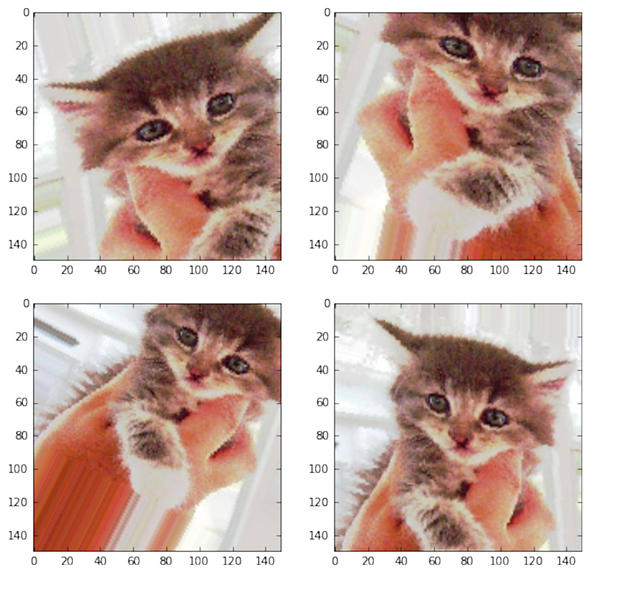
Fig: generating cat pictures using data augmentation
The networks will never receive the same inputs twice if you train a new network using a data-augmentation setting. However, because it only receives inputs from a tiny number of original photos, those inputs are still highly linked; you can only remix already-existing information. As a result, this might not be sufficient to eradicate overfitting. You should include a Dropout layer in your algorithm before densely linked classifier to combat overfitting further.
Data Augmentation Applications in Real-time
1. Healthcare
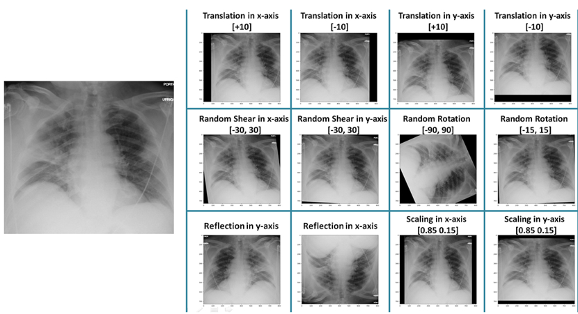
Curating datasets is not a solution for medical imaging applications because getting a lot of expertly labelled samples takes a long time and money. The network designed by augmentation must be more reliable and authentic than the predicted shifts in similar X-Ray pictures. However, we can increase the dataset number in the subsequent illustration by employing data augmentation.

Fig: Data augmentation in X-Ray image
2. Self-driving cars
Autonomous vehicles are a different use topic where data augmentation is beneficial. For example, CARLA was designed to generate flexibility and realism in the physics simulation. CARLA was created from the initial idea to promote the autonomous driving system’s outcome, instruction, and validation. It is based on Unreal Engine 4 and offers a complete simulator environment for testing autonomous driving technologies in a safe setting.
When data scarcity is a problem, simulation environments created employing reinforcement learning techniques can aid in the training and testing of AI systems. The ability to model the simulated environment to create real-life scenarios opens up a world of possibilities for data augmentation.
Defining the CNN Model from Scratch
####------Defining CNN, including dropout--------####
model = models.Sequential()
model.add(layers.Conv2D(32, (3, 3), activation='relu', input_shape=(150, 150, 3)))
model.add(layers.MaxPooling2D((2, 2)))
model.add(layers.Conv2D(64, (3, 3), activation='relu'))
model.add(layers.MaxPooling2D((2, 2)))
model.add(layers.Conv2D(128, (3, 3), activation='relu'))
model.add(layers.MaxPooling2D((2, 2)))
model.add(layers.Conv2D(128, (3, 3), activation='relu'))
model.add(layers.MaxPooling2D((2, 2)))
model.add(layers.Flatten())
model.add(layers.Dropout(0.5))
model.add(layers.Dense(512, activation='relu'))
model.add(layers.Dense(1, activation='sigmoid'))
model.compile(loss='binary_crossentropy', optimizer=optimizers.RMSprop(lr=1e-4), metrics=['acc'])
Let’s train the network using data augmentation and dropout.
####-------Train CNN using data-augmentation--------#####
train_datagen = ImageDataGenerator(rescale=1./255, rotation=40, width_shift=0.2, height_shift=0.2, shear=0.2, zoom=0.2, horizontal_flip=True,)
test_datagen = ImageDataGenerator(rescale=1./255)
train_generator = train_datagen.flow_from_directory(train_dir, target_size=(150, 150), batch_size=32, class_mode='binary')
validation_generator = test_datagen.flow_from_directory(validation_dir, target_size=(150, 150), batch_size=32, class_mode='binary')
history = model.fit_generator(train_generator, steps_per_epoch=100, epochs=100, validation_data=validation_generator, validation_steps=50)
####-------Save the model--------#####
model.save('cats_and_dogs_small_2.h5')
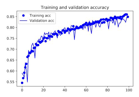
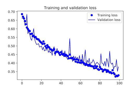
You are no longer overfitting because of data augmentation and dropout. Because the training and validation curves near correspond to each other. With this accuracy, you surpass the non-regularized model by 15% and achieve 82%. Let’s plot the curves;
Displaying Curves of Loss and Accuracy During Training


You may achieve even higher accuracy, up to 86% or 87%, by using other regularisation approaches and fine-tuning the network’s parameters (such as the number of filters per convolution layer or the number of layers in the network). However, because you have small data to work with, it would be challenging to achieve higher levels simply by training your own CNN from scratch.
You must employ a pretrained model as a further step to increase your accuracy on this challenge.
In my next blog, I will describe how to train the pretrained model for your work.
Conclusion
- Training data’s quality, volume, and contextual essence significantly affect deep learning models’ accuracy. But one of the biggest problems in developing deep learning models is a lack of data.
- Acquiring such data might be expensive and time-consuming in production use methods. Companies use data augmentation, a low-cost and efficient technique, to develop high-precision AI models more quickly and lessen reliance on gathering and preparing training instances.
- This article explains how we can use data augmentation techniques to train our model. When collecting vast amounts of data is challenging, data augmentation is utilized. As discussed in the blog, healthcare and driverless cars are two of the most well-known sectors using this approach.
The media shown in this article is not owned by Analytics Vidhya and is used at the Author’s discretion.


