This article was published as a part of the Data Science Blogathon.
Introduction
In today’s world, the demand for machine learning and artificial intelligence is increasing, with more companies developing computer systems and building new technologies to achieve this goal. AI has become the world’s fastest-growing technology, with an estimated total of over 30,000 new machines per day. Object Detection and Object Classification are a part of AI, which are also significantly trending these days. Self-driving cars are gaining popularity nowadays. These cars can detect objects on the road in real-time by using these highly efficient object detection models. Also, using intelligent driving technology to detect pedestrians is becoming a popular industry with some companies such as Tesla.
In this article, we will create an image classification model using convolutional neural networks capable of classifying the images in 10 different classes. We will also discuss the accuracy and loss curves of the trained model on the test set.
Analysis of Dataset:
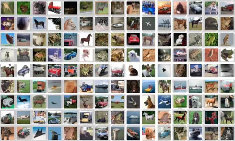
CIFAR-10 dataset comprises 60,000 32×32 colour images, each containing one of ten object classes, with 6000 images per class. It consists of 50,000 32×32 color training images labelled across ten categories and 10,000 test images.
In the case of the CIFAR-FS dataset, the train-test-split is 50000 samples for training and 10000 for testing as well. The size of the image is 32*32*3.
Different Classes present:
['airplane', 'automobile', 'bird', 'cat', 'deer', 'dog', 'frog', 'horse', 'ship', 'truck']
Number of samples of different classes in each of the testing and training dataset
train_dataset class : {'frog': 5000, 'truck': 5000, 'deer': 5000, 'automobile': 5000, 'bird': 5000,
'horse': 5000, 'ship': 5000, 'cat': 5000, 'dog': 5000, 'airplane': 5000}
test_dataset class : {'cat': 1000, 'ship': 1000, 'airplane': 1000, 'frog': 1000, 'automobile': 1000,
'truck': 1000, 'dog': 1000, 'horse': 1000, 'deer': 1000, 'bird': 1000}

Implementation
Loading and Pre-Processing of Dataset: In this section, we will see the code for loading and pre-processing the Cifar-10 dataset. Firstly, we will download the dataset directly using the torchvision library and divide the dataset into training and testing sets.
train_dataset = torchvision.datasets.CIFAR10(root='data/', train=True, download=True, transform = transforms.ToTensor())
test_dataset = torchvision.datasets.CIFAR10(root='data/', download=True, train=False, transform = transforms.ToTensor())
torch.manual_seed(42)

my_list = [45000,5000]
train_ds, val_ds = torch.utils.data.random_split(train_dataset, my_list)
configs = {‘random_seed’ : 42, ‘val_size’ : 5000, ‘train_size’ : 45000, ‘pin_memory’:True,’optimizer’:’Adam’,’batch_size’:64,’lr’:0.001 }
Check GPU Availability: We will check whether our system contains a dedicated GPU or not. GPU speeds up our training process, as it contains special hardware.
def GPU_IsAvailable():

    if torch.cuda.is_available():

        temp = torch.device('cuda')

        return temp

    else:

        tmp1 = torch.device('cpu')

        return tmp1
Some Basic Functions: Below, some basic functions are written, like evaluate, which is used to evaluate the model’s accuracy on the test data. And another function named fit is used the fit the training data inside the CNN model.
channel = 3

num = 28

@torch.no_grad()

def evaluate(model, val_loader, dt_load):

    model.eval()

    outputs = []

    for i in val_loader:

      temp = model.val_func(i, num, channel)

      outputs.append(temp)


    var3 = model.valid_func(outputs, num)

    return var3


def fit(epochs, lr, model, train_loader, val_loader):

    lst1 = list()

    lst2 = list()

    opt_func = optim.Adam

    optimizer = opt_func(model.parameters(), lr)

    for epoch in range(epochs):

        lst3 = []

        # Training Phase

        model.train()

        for batch in train_loader:

            loss = model.train_func(batch, num)

            lst3.append(loss)

            loss.backward()

            optimizer.step()

            optimizer.zero_grad()

        # Validation phase

        result = evaluate(model, val_loader, epc)

        result['train_loss'] = torch.stack(lst3).mean().item()

        model.func(epoch, result, channel)

        lst1.append(result)

    return lst1
Defining the CNN Model: Our CNN models will contain three layers containing one convolutional layer and one max pooling layer.
two = 2

one=1

class CnnModel1_2(Class1):

    def __init__(self):

        super().__init__()

        self.network = nn.Sequential(

            nn.Conv2d(dims, 32, kernel_size=dims, stride=one, padding=one),

            nn.ReLU(),

            nn.MaxPool2d(two, two),


            nn.Conv2d(32, 64, kernel_size=dims, stride=one, padding=one),

            nn.ReLU(),

            nn.MaxPool2d(two, two),


            nn.Conv2d(64, 128, kernel_size=dims, stride=one, padding=one),

            nn.ReLU(),

            nn.MaxPool2d(two, two),


            nn.Flatten(),

            nn.Linear(4*4*128, 10))


    def forward(self,x):

      x = self.network(x)

      return x
Training of Model: We will set the number of epochs to be 20 and then for the training data into the model
model1_2 = CnnModel1_2()
train_data1_2 = Data_loader(GPU_IsAvailable(), train_data)

val_data1_2 = Data_loader(GPU_IsAvailable(), val_data)
GPU_Calculate(model1_2, GPU_IsAvailable())
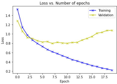
Plotting the loss v/s no. of epochs curve:
import matplotlib

train_losses = [x.get('train_loss') for x in history]

val_losses = [x['val_loss'] for x in history]
matplotlib.pyplot.plot(train_losses, '-bx')

matplotlib.pyplot.plot(val_losses, '-yx')

matplotlib.pyplot.xlabel('Epoch')

matplotlib.pyplot.ylabel('Loss')

matplotlib.pyplot.legend(['Training', 'Validation'])

matplotlib.pyplot.title('Loss vs. Number of epochs')

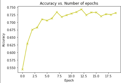
Plotting the accuracy v/s no. of epochs curve:
accuracies = [x['val_acc'] for x in history]
matplotlib.pyplot.plot(accuracies, '-yx')
matplotlib.pyplot.xlabel('Epoch')
matplotlib.pyplot.ylabel('Accuracy')
matplotlib.pyplot.title('Accuracy vs. Number of epochs');

Discussions
Q. How does changing the network size change the accuracy?
As we know, the Convolutional neural network consists of two main components, i.e., feature extraction and classification. So, in these types of networks, convolution operations are doing the task of feature extraction, whereas fully connected layers will do the job of classification.
We observe that on changing the network size from three experimentations from I to iii, the accuracy tends to improve, which is evident from the fact that varying the network sizes affected accuracy. However, on the contrary, it has been observed that two FC layers are present in the case of the third architecture.
Q. Experiment with different pooling sizes and do a detailed analysis of pooling size on the network.
As we know, pooling is a user-defined operation. We have different types of pooling in hand, such as Max pooling, sum pooling, and average pooling, with their pros and cons. Still, in general, we are using Max pooling as it will perform better on a given problem statement as we’re trying to extract the features based on their importance. Because it contained more feature extraction layers, the dual convolution blocks (Conv-Conv-Pool-Conv-Conv-Pool) fared better than the other models. Its distinguishing power grew, allowing it to function better. We also revealed that adding more than one FC layer did not affect performance, implying that adding additional FC layers does not guarantee better performance. It is more reliant on the feature extraction layers. When we increase the pooling size, one of the two things occurs, i.e., either we get more generalizability, or some essential features are lost as more shrinking occurs.
Q. How the presence of one or more fully connected layers changes the accuracy?
Based on the experimentation done in one of the research papers on Neurips, it has been observed that one fully connected layer is necessary for the proposed architecture for doing the task of classification as the FC layer will do the job of classification, similar to what we have done in artificial neural networks. With the presence of one of the more fully connected layers, accuracy increases a lot. The reason is that the functionality of fully connected layers is to classify while that of convolution layers is to extract features. Their presence makes classification better and increases accuracy.
Conclusion
You can download the complete code from this link.
This article discusses how we can create an image classification model using Convolutional Neural Networks, Cifar-10 dataset. CNN can use image classification for various applications like cancer detection or biometric authentication. CNN works well with the data, which has some spatial relationship. It automatically detects important features from images without any human intervention.
Despite these advantages, there are some disadvantages also of CNN, requiring high computational power, extensive training data, overfitting of the training data, etc.
Key takeaways of this article:
1. We have discussed the Cifar-10 dataset. We have found that this dataset contains a total of 60000 images of size 32×32 for ten different classes like a bird, cat, dog, deer, etc.
2. After that, we discussed dataset loading and pre-processing. In this, we have downloaded the dataset directly from the torchvision library. After that, we split the data into training and testing sets.
3. Then, we trained our model using CNN. In this, we first checked the availability of GPU in our machine. After that, we made a pipeline of several CNN layers, and after training the model, we found the loss and accuracy curves.
The media shown in this article is not owned by Analytics Vidhya and is used at the Author’s discretion.


