Simple framework to build a survival analysis model on R

In the last article, we introduced you to a technique often used in the analytics industry called Survival analysis. We also talked about some of the application of this technique across the industries. In this article we will layout a simple framework to use survival analysis on the tool R.

[stextbox id=”section”] Case Study (Background)  [/stextbox]

You are the head of the analytics team with an online Retail chain Mazon. You have received a limited number of offers which costs you $200/customer targeted . The offer breaks even if a customer makes a purchase of minimum $20,000 in his entire lifetime. You want to target customers who are likely to make a purchase of $20,000 as early as possible. You have their relationship card segment (Platinum cards are expensive and Gold card is cheaper) and their response rate on last campaign they were targeted with. You have been targeting customers with this offer for past 1 year. Now you want to learn from the past response data and target accordingly. You need to find which customer base should you target for this offer. You will have to use survival analysis in this case because the dependent variable is the time to respond the campaign. This again contains censored data which are people who did not respond till date.

[stextbox id=”section”] Data Structure [/stextbox]

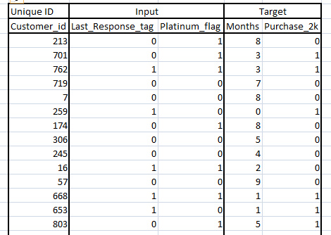
 The raw data includes a unique ID, 2 input variables and 2 target variables. The first target variable is months, which indicates the number of months customer has not completed a total purchase of $20,000.  The second target variable is Purchase_2k, which indicates if the customer finally makes a purchase of $20,000. Any customer who have not yet made the purchase is not a non-responder but a censored data.

Censored data is an observation for whom the actual response tag is unknown. Say, customer id “213” made a purchase of $19,999 till month 8 when the data was collected. His month variable will have a value of 8 and Purchase_2k will have a value of 0. But the next day, customer 213 completed $20,000. Hence, on the date of collection this data should not be treated as a non-responder but a censored observation. Other direct techniques like logistic regression cannot take censored data into the model. However, survival analysis has a capability to take them into account.

[stextbox id=”section”] Theory behind Survival analysis (Optional read) [/stextbox]

Survival and hazard functions : Survival analysis is modelling of the time to death. But survival analysis has a much broader use in statistics. Any event can be defined as death. For example, age for marriage, time for the customer to buy his first product after visiting the website for the first time, time to attrition of an employee etc. all can be modeled as survival analysis.

Let’s say T is a random variable which signifies the variable time. We define the function f(t) as the probability distribution function (pdf) on this random variable. F(t) is the cumulative distribution function with F(t) = Pr { T < t }.  Now the survival function S(t) is mathematically written as follows :

Finally, we define a Hazard function (instantaneous rate of occurrence of the event) mathematically as follows :

From the above relationships, it is clear that if one of the Survival function, pdf or Hazard function is known, others can be calculated easily. To estimate these functions we have three kinds of solutions. Following are the three ways of estimation :

1. Non-parametric solution : Simplest solution which can be used for descriptive analysis, but cannot be extrapolated to find out the survival of censored data with high time span.

2. Semi – Parametric solution : Widely used in the industry.  Will be discussed in detail in this article.

3.  Parametric solution : We will not touch up on this route of estimation. The reason being the parameters found by different software have different signs. We will cover this in one of the coming articles.

[stextbox id=”section”] Solving survival analysis on R ( Initializing)  [/stextbox]

To model survival analysis in R, we need to load some additional packages. Following are the initial steps you need to start the analysis.

Step 1 : Load Survival package

Step 2 : Set working directory

Step 3 : Load the data set to the temporary memory of R

> library(survival)

> setwd (“D:/”)

> mydata <- read.csv (“D:/worksheet.csv”)

> attach(mydata)

Once we have data in our temporary memory, you need to create an array of input variable. Note that, till this point both non-parametric and semi-parametric have the same standard codes. We will use different codes for the two later in the process.

> Cust <- Customer_id
> l_resp <- Last_Response_tag
> Plat <- Platinum_flag
> span <- Months
> Resp <- Purchase_2k
> X <- cbind(l_resp,Plat)

Here, we have clubbed the input or defining functions. Also note that span and Resp are both target functions.

[stextbox id=”section”] Non-parametric solution [/stextbox]

Non-parametric solution to survival analysis problem gives a directional view on which profile has a better survival rate. It cannot be extrapolated to higher time span predictions. Use following steps to create a survival curve and get insights to the overall portfolio survival view.

> kmsurv <- survfit(Surv(span,Resp) ~ 1)
> summary(kmsurv)
> plot(kmsurv,xlab = “span”,ylab=”Survival Proabability”)

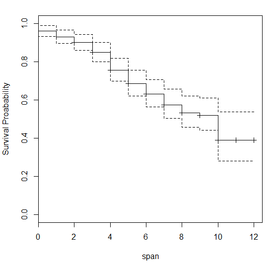
Above is the graph we get after executing the codes. Let’s try to understand this curve. This is a survival curve, which shows following facts about the population:

1. The curve starts from a point below 1, which means some of the observation/customer made an immediate purchase of $20,000 just after receiving the offer (in month 0)

2. After 6 months, around 62% of the population have survived. In other words, 38% of the population has made a purchase of more than $20,000

3. Around 38% of the population survives even after 12 months. This does not mean they will never make a purchase. But from a non-parametric solution we cannot extrapolate the solution for more than 12 months.

To make a deep-dive into this population, lets look at the survival curve of individual strata. Strata are different levels of input variable for the population.In this case study, we have 2 levels of 2 input variables.

1st variable (Response of last time) : Any individual customer will either have responded in the last offer or not. Hence, this variable has two levels.

2nd variable (Membership) : There are two types of membership which we offer. Either a customer can be Gold or Platinum. Again, this variable has two levels.

Execute following code to get survival curves on these individual levels.

> group1 <- l_resp

> group2<- Plat

> kmsurv1 <- survfit(Surv(span,Resp) ~ group1)
>  summary(kmsurv1)
>  plot(kmsurv1,xlab = “span”,ylab=”Survival Proabbility”)

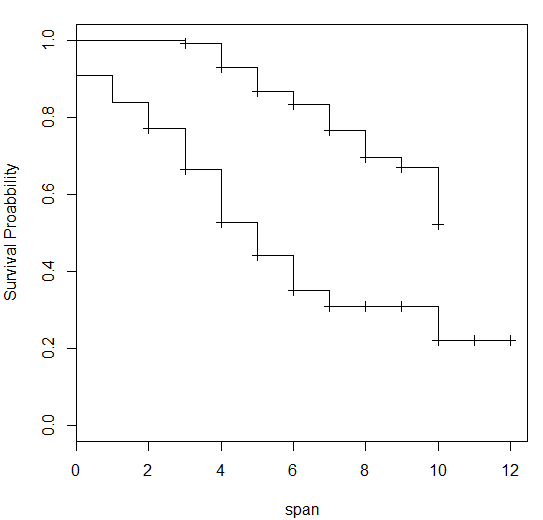
Above is the curve you get on execution of the code. Note that curve with higher values of probability is for group1 =0 or non-responders of last campaign. Hence we can infer from this graph that non-responders of last campaign have a higher probability to not respond for this campaign as well compared to rest at any point of time till 12 months. We can do a similar exercise for package. Here again we find customer with Platinum package has a higher probability to make a purchase of $20,000 in any number of months till 12 months.

[stextbox id=”section”] Semi-parametric solution [/stextbox]

Cox(1972) introduced an approach which directly focuses on estimating the hazard function directly using both time and profile variables. Following is the equation for hazard which we want to solve :

Here is the code you need to write to execute Cox hazard model.

coxph <- coxph(Surv(span,Resp)~X,method = “breslow”)

summary(coxph)

Let’s try to understand the output step by step.

1. Data summary :  The first line of the output summarizes the entire data. In total we have 199 observation out of which for 84 observations, the event has already occurred.

2. Coefficient estimates: These estimates help us understand the impact of profile on survival rate. As you can see, for both the variables p value is low and, hence, both the variables are significant. Also both of them have a positive sign which implies two facts about the population :

1. Platinum customers have a higher probability of making a purchase of more than $20,000

2. Last campaign responders have a higher probability of making a purchase of more than $20,000

3. Marginal effect table : This table does not have anything new compared to table 2. But, it teller you the % increase in the risk of event happening (which in this case is a good thing) by unit increase in input variable (which in this case are only two level variables).  Hence, following are the insights coming out of this table :

1.  Platinum customers have 230% higher chance to make a purchase of more than $20,000.

2.  Last campaign responders have 290% higher chance to make a purchase of more than $20,000.

[stextbox id=”section”]End Notes [/stextbox]

Survival analysis provides a solution to a set of problems which are almost impossible to solve precisely in analytics. These solutions are not that common at present in the industry, but there is no reason to suspect its high utility in the future. In this article we covered a framework to get a survival analysis solution on R. In one of our future articles, we will also cover doing survival analysis in SAS.

Did you find any opportunity in your line of business where you can implement survival analysis? Did you find this article helpful? Have you worked on other cutting edge modelling techniques in the recent past? Were the results encouraging? Do let us know your thoughts in the comments below.

If you like what you just read & want to continue your analytics learning, subscribe to our emails, follow us on twitter or like our facebook page.

Tavish Srivastava

Tavish Srivastava, co-founder and Chief Strategy Officer of Analytics Vidhya, is an IIT Madras graduate and a passionate data-science professional with 8+ years of diverse experience in markets including the US, India and Singapore, domains including Digital Acquisitions, Customer Servicing and Customer Management, and industry including Retail Banking, Credit Cards and Insurance. He is fascinated by the idea of artificial intelligence inspired by human intelligence and enjoys every discussion, theory or even movie related to this idea.