Predictive Models play an important role in the field of data science and business analytics, and tend to have a significant impact across various business functions. Building such models is often a very iterative process that involves lots of trials depending on the data size in terms of observations and variables. Most common problems that predictive models can solve fall under regression and classification categories, and various techniques that can be implemented range across least squares regression, logistic regression, tree based models, neural networks and support vector machines. In model building process, initially it is recommended to perform all the iterations one by one to get a good grasp on the underlying concepts. After building some expertise, then probably one can think of considering more automation as a substitute for model iterations.
The “caret” package in R is specifically developed to handle this issue and also contains various in-built generalized functions that are applicable to all modeling techniques. Let us look at some of the most useful “caret” package functions by running a simple linear regression model on “mtcars” data. This article would focus more on how various “caret” package functions work for building predictive models and not on interpretations of model outputs or generation of business insights.
Data Loading and Splitting:
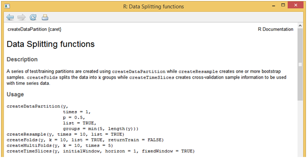
For this sample project, we will make use of in-built dataset named “mtcars” in R. After loading the data, one of the first tasks that needs to be performed, is to split it into development and validation samples. Using “createDataPartition” function present in “caret” package, data split task can be performed easily. Syntax and other parameters supported by this function can be accessed by running the below function in R console.
[stextbox id = “grey”]??createDataPartition
[/stextbox]And let’s say development sample would 80% of observations in “mtcars” data and remaining observations into the validation sample.
[stextbox id = “grey”]
library(caret)
library(datasets)
data(mtcars)
split<-createDataPartition(y = mtcars$mpg, p = 0.6, list = FALSE)
dev<-mtcars[split,]
val<-mtcars[-split,]
Model Building and Tuning:
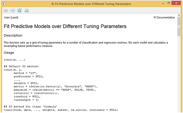
The train function can be used to estimate coefficient values for various modeling functions like random forest and others. This function sets up a grid of tuning parameters and also can compute resampling based performance measures.
[stextbox id = “grey”]
?train
[/stextbox]As per this example, let us build a linear regression model that uses least squares approach to determine optimal parameters for the given data. The following R script showcases the syntax needed to build a single model where all the variables are being introduced.
[stextbox id = “grey”]
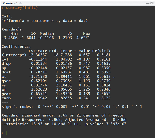
lmFit<-train(mpg~., data = dev, method = “lm”)
summary(lmFit)
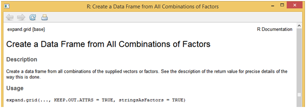
If you want to use a different modeling function, all it takes is to change the respective model name in the method parameter of “train” function. Say for logistic regression model the method will take “glm”, for random forest model the method will take “rf” and soon. Generally, model building will not be complete in single iteration and often needs more trails. This can be achieved by using the “expand.grid” function which will be more useful especially with advanced models like random forest, neural networks, support vector machines etc.
[stextbox id = “grey”]
?expand.grid
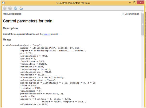
[/stextbox]Another useful function would be “trainControl” which allows for estimation of parameter coefficients through resampling methods like cross validation, boosting etc. While using these parameters, then entire data can be used for model building without splitting it. Below script showcases the use of cross validation technique and also how to apply it on the loaded data using “trainControl” function.
[stextbox id = “grey”]
?trainControl
[/stextbox]
[stextbox id = “grey”]
ctrl<-trainControl(method = “cv”,number = 10)
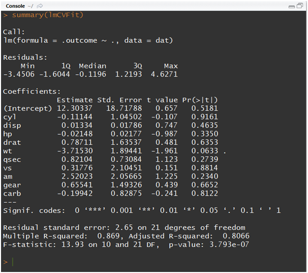
lmCVFit<-train(mpg ~ ., data = mtcars, method = “lm”, trControl = ctrl, metric=”Rsquared”)
summary(lmCVFit)
Model Diagnostics and Scoring:
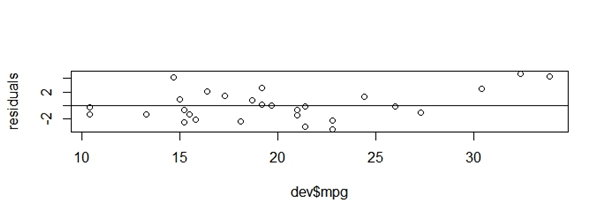
Once the final model is identified, as a next step one should compute model diagnostics which would vary depending on the modeling technique used. Say for linear regression model, the standard diagnostics tests are residual plots, multicollinearity check and plot of actual vs predicted values. These would vary for logistic regression model such as AUC value, classification table, gains chart etc. Below script showcases R syntax for plotting residual values vs actual values and predicted values vs actual values.
[stextbox id = “grey”]
residuals<-resid(lmFit)
predictedValues<-predict(lmFit)
plot(dev$mpg,residuals)
abline(0,0)
plot(dev$mpg,predictedValues)
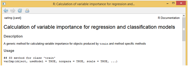
One of the most useful functions would be “varImp” which showcases variable importance of the variables used in the final model.
[stextbox id = “grey”]??varImp
[/stextbox]varImp(lmFit)
plot(varImp(lmFit))
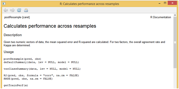
Finally, scoring needs to be performed on the validation sample or any other new data using the parameter estimates obtained from the model building process. This step can be easily implemented with the help of “predict” function. Below script showcases how the scoring task is performed on the val sample using the coefficients obtained from the model built on dev sample. And in order to see the model performance metrics on validation sample, a function “defaultSummary” can be used which in this example returns the values of R-squared and RMSE metrics.
[stextbox id = “grey”]
??defaultSummary
[/stextbox]predictedVal<-predict(lmFit,val)
modelvalues<-data.frame(obs = dev$mpg, pred=predictedVal)
defaultSummary(modelvalues)
So far, we have looked at some of the useful functions as part of “caret” package that can be used for building predictive models in R. As we have noticed, this package implements a general class of in-built functions that can be used across all modeling techniques. You can learn more about this package and its functions from the below references.
Building Predictive Models in R using the caret Package
The caret Package: A Unified Interface for Predictive Models
 Kiran is a graduate of IIT-Madras with more than five years of professional experience in business analytics. He is currently a faculty at Jigsaw Academy. Prior to Jigsaw, he worked at LatentView Analytics delivering advanced analytics and business consulting solutions to various clients across verticals such as E-Commerce, Insurance, Technology and Financial Services. He has strong proficiency in working with tools such as SAS, R, MySQL, Python, Hadoop, Tableau etc. In free time, he enjoys participating in data mining contests on open platforms like Kaggle and CrowdAnalytix.
If you like what you just read & want to continue your analytics learning, subscribe to our emails, follow us on twitter or like our facebook page.


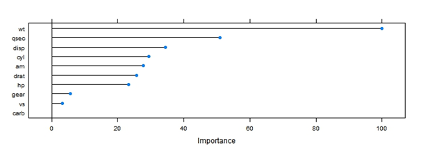


You need to set seed for reproducibility Try set.seed(123) and set.seed(234) before data partion You will see a different solution when you plot variance importance with plot(varImp(lmFit)) The reason is that the partiton at 60/40 randomly includes different type of cars, with a different role of the variables
Good point Antonello
why are the regression results the same for the baseline model and the cross-validated model?? Shouldn't cross validation improve or at least change the results?
Good One
Glad you like the article!