Introduction
Survival analysis is one of the less understood and highly applied algorithm by business analysts. That is a dangerous combination! Not many analysts understand the science and application of survival analysis, but because of its natural use cases in multiple scenarios, it is difficult to avoid!
P.S. If you read the first half of this article last week, you can jump here. We have combined the articles to make it more useful for our readers.
Survival analysis refers to analyzing a set of data in a defined time duration before another event occurs. The number of years in which a human can get affected by diabetes / heart attack is a quintessential of survival analysis. Survival analysis is one of the most used algorithms, especially in Pharmaceutical industry.
In one of the previous article, we have already discussed the use cases of survival analysis. We also talked about non-parametric and semi-parametric survival analysis. We suggest you to go through these articles first to get a good understanding of this article.
In this article, you will learn:
- The basics of Parametric analysis to derive detailed and actionable insights from a Survival analysis.
- How to find the right distribution in a parametric survival model?
- Different functions used in parametric survival model followed by their applications.
Let us first understand how various types of Survival analysis differ from each other.
Basics of Survival analysis
A survival analysis is different from traditional model like regression and classification problems as it models two different parameters. To understand the Survival analysis in detail, refer to our previous articles(1 & 2). However, in this article we will also discuss how the three types of analysis are different from each other.
The image above will help you understand the difference between the three classes of Survival analysis models. Having already explained about semi parametric models, we will go a step ahead and understand how to build a Parametric model.
In a parametric model, we assume the distribution of the survival curve. Even before fitting a model, you need to know the shape of the Survival curve and the best function which will fit in this shape. For this you need to build a non-parametric model and understand the shape of hazard function and the survival curve.
What are the distributions used in Parametric Models?
There are five types of distribution of Survival/hazard functions which are frequently assumed while doing a survival analysis. The name of each of these distribution comes from the type of probability distribution of the failure function. Following are the 5 types of probability distribution curve generally used in parametric models. Each distribution been explained below in detail:
- Normal Distribution
- Uniform Distribution
- Exponential Distribution
- Weibull Distribution
- Lognormal Distribution
For each of these distributions, let’s first understand the following plots :
1. Lifetime Distribution Function (F) : This is the probability of failure happening before a time ‘T’.
2. Lifetime Probability distribution (f) : A differential of F will give us probability distribution. All the names of distribution function is based on this probability distribution.
3. Survival Function (S) : Survival is the inverse of Lifetime. It is one minus Lifetime distribution.
4. Hazard Function (Lambda) : Hazard function is the rate of event happening. Hazard function can be derived from the Survival function as follows :
5. Cumulative Hazard Function : This is simply the integral of the hazard function and is given as below :
Also, by integrating the hazard function equation we get following equation :
Following are the two plots we will refer in each case (these are the important ones to select the distribution) :
a. Hazard Function
b. Survival Function
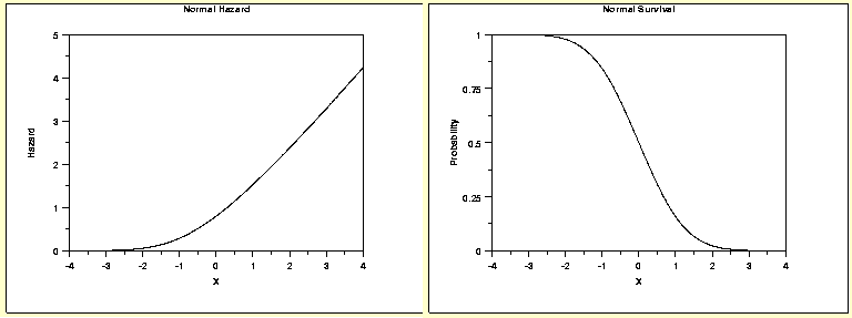
1. Normal Distribution
This type of distribution is assumed when the risk of failure increases considerably with time. Hence, the probability of failure increases suddenly. Check the graphs shown below:
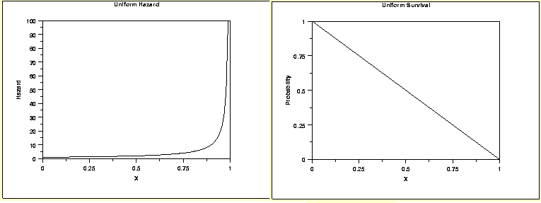
2. Uniform distribution
Uniform distribution is not a common type to be assumed in real world. The survival curve is just a straight line from 100% to 0%. And the hazard function increases exponentially to force death of every single observation towards the end. Check the graphs shown below:
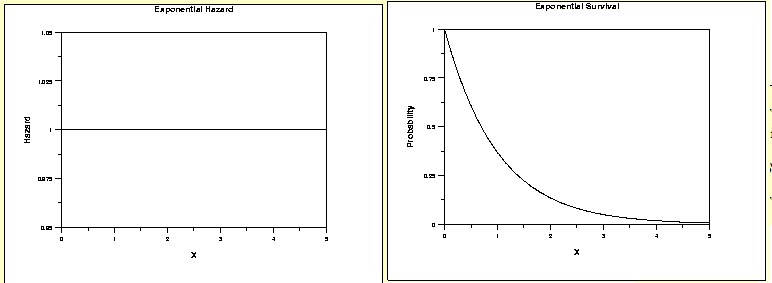
3. Exponential Distribution
Exponential distribution is one of the common assumption taken in survival models. The hazard function does not vary with time. This distribution can be assumed in case of natural death of human beings where the rate does not vary much over time. Check the graphs shown below:
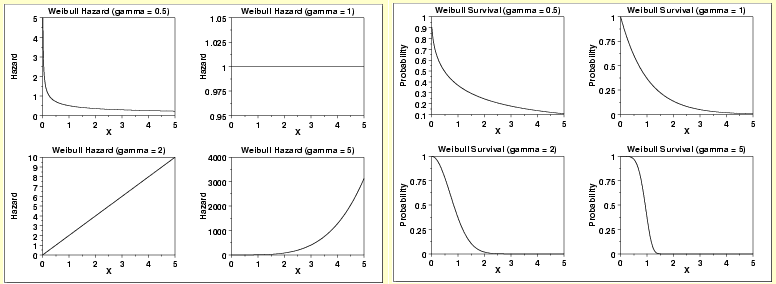
4. Weibull Distribution
Weibull distribution has a parameter gamma which can be optimized to get different distributions of hazard function. Following are a few scenarios which will illustrate the same:
As you can see from the multiple scenarios, gamma can change the weibull hazard function from steep decline to constant function to accelerating increase. Hence, it fits into multiple situations in our practical world.
5. Log-normal Distribution
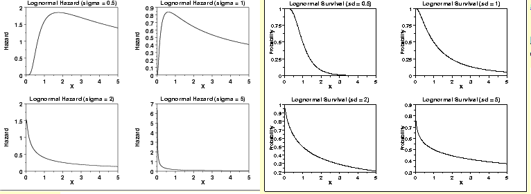
Here is another distribution which can be optimized for different hazard functions. Lognormal distribution can be complimented by Weibull distribution to simulate almost every scenario. Check the scenarios as shown below:
As you can notice from the above graphs: With changing value of sigma, the curve changes its nature. This function can generate non-monotonic natures of hazard function. This is a single scenario where weibull curve does not fit well. Hence, they both complement each other well and literally can be used for all scenarios.
What are the applications of Survival Analysis?
To understand the applications, let’s now take a step back and think of cases where Survival analysis can be used and based on the expected distribution fit the best possible curve.
Assignment : Before looking at the answers try to attempt the best fit distribution in each case.
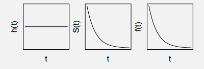
Case 1 : Time until next case of scientific innovation.
Because innovations are not biased towards any specific reasons, the hazard function is a constant line. Hence, following are the Hazard Function, Survival function and the probability distribution function:
Case 2 : Life of patients of Cancer who are not responding to any treatment
Cancer gets worse with time and hence the survival rate deteriorates much faster. Following are the Hazard Function, Survival function and the probability distribution function:
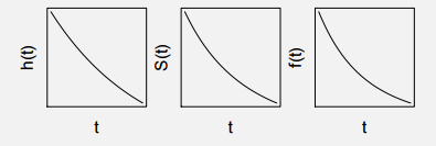
Case 3 : Life of a patient after surgery OR Financial state of a country/company after a big shock
Whenever there is a deteriorating effect shock. For example: Condition of patients after surgery where the risk of anything turning unfavourable, goes down with time. Below we have following type of the Hazard Function, Survival function and the probability distribution function:
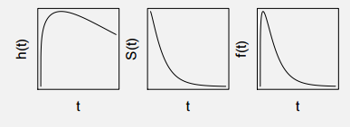
Case 4 : Life of a patient recently detected with Swine Flu or TB
Diseases like Swine Flu or TB have a sharp impact. If the patient can survive the initial period of these diseases, the danger of death gradually subsides as the time passes on. Following are the Hazard Function, Survival function and the probability distribution function:
The right distribution for each case:
Now let’s think over what distribution fits well in each of these cases:
Case 1 : Both Exponential and Weibull can be used for this case as hazard function is a constant curve.
Case 2 : Weibull function with gamma = 2 can be used as the hazard function is a linearly increasing curve.
Case 3 : This is kept as an assignment for this article. You won’t find a direct answer in this article but with a good basic understanding, you should have no challenge figuring this out.
Case 4 : This is the classic case of the use of Log normal distribution. The hazard function shows a peak and hence the log-normal with sigma less than 1 is suitable for this case.
End Notes
This article will help you understand the Survival analysis. It also explains how to estimate distributions given the survival plots. People generally miss out on understanding the application of any concept they choose to learn. In this article, we have also discussed various cases which describes the diverse applications of this Parametric Analysis. Case 3 is given as an assignment. Write your detailed answers in the box below.
Were you haunted by any questions/doubts while learning this concept? Don’t worry, ask our analytics community and never let your learning process stop by any of the hurdle which comes across your way!
Did you find the article useful? Do let us know your thoughts about this guide in the comments section below.


