Getting Mongo-ed in NoSQL manager, R & Python

Introduction

I started my journey on Analytics Vidhya (AV) as a follower. AV, and now especially the discussion portal, always stay open in one of the windows of my working machine. Like thousands of you, who read and love these resources, I owe a lot of my learning in Analytics career to Analytics Vidhya. This relationship evolved further, when my previous article on Beginners Guide to MongoDB gave me a glimpse of what the platform can do for people like me.

I am basking in the glory of this new found love with my old companion / mentor and taking this journey of contributing back to the community a step forward. In this article, I explain how to use MongoDB in NoSQL Manager, R and Python.

Integration of MongoDB with analytics tools:

MongoDB is the most popular NoSQL database out there. It is used by several big companies like ebay, Criagslist, FourSquare etc. Most of the popular data analysis tools like R and Python offer incredible packages to integrate themselves with MongoDB. These packages enable people to use Mongo & its powerful features from the windows of their choice and comfort.

Some of the popular packages integrating MongoDB to the analytics tool are RMongo, PyMongo, Mongolite, JSON Studio and jSonarR.

Here is a brief introduction of these packages:

1. PyMongo – As the name suggests, this is the essential set of tools necessary to work with MongoDB in Python.
2. RMongo – It is popularly known as a MongoDB client and provides a database interface for R. The interface is provided via Java calls to the Mongo-Java-driver.
3. Mongolite – It is another MongoDB client for R but is faster and simpler to use. This package is based on ‘jsonlite’ and ‘mongoc’ driver. Furthermore, it includes support for aggregation, indexing, map-reduce, streaming, ‘TLS’ encryption and ‘SASL’ authentication.
4. JSON Studio – JSON Studio provides easy accessibility to the data stored as JSON in MongoDB. It is used by anyone who wants to view, analyze, visualize or slice-and-dice data in MongoDB. It consists of eight applications. Few of them are: aggregation builder, spreadshet bridge, SQL transfer, schema analyzer.
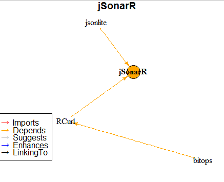
5. jSonarR – This package runs queries and returns their result in R data frames, thereby allowing users to access MongoDB. It converts the JSON document format to a tabular form which makes it easy to use with existing R packages.

Structure of the remaining article:

I have structured this article in four parts as described below. We first look at how various operations can be performed using NoSQL manager and then see various packages in R and Python.

1. CRUD operations & Aggregation in MongoDB using NoSQL Manager.
2. Using the “RMongo” & “Mongolite” package in R.
3. Using “PyMongo” in Python.
4. Using JSON studio and “jSonarR” package in R.

1. CRUD operations & Aggregation in MongoDB using NoSQL Manager

CRUD stands for: C – Create, R – Read, U – Update, D – Delete. On the other hand, aggregation operations process data records and return computed results. Understanding how these operations can be performed using NoSQL manager would lay the foundation for the remaining article. Once we know this, we will perform similar operations from R and Python.

MongoDB stores data in the form of documents: JSON-like field and value pairs called BSON. In the documents, the value of a field can be any of the BSON data types, including other documents, arrays, and arrays of documents. We’ll perform various CRUD and aggregation operation sequentially.

1.a) CREATE

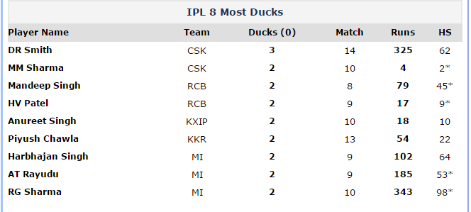
We will create two collections namely IPL (Indian Premier League) Fastest Century and IPL Most Runs. Please note that I am calling these collections (and not tables) and I would suggest all wannabe Mongo-ers to do so as well.

1. IPL_Fastest_Century

                                                          (IPL 8 – Indian Premier League Season 8)

2. IPL_Most_Runs

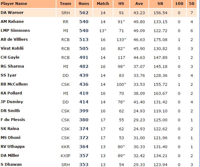
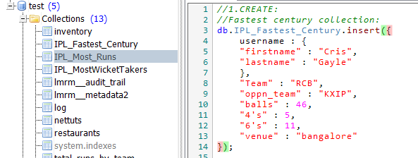
Now we’ll insert these records in the database. Here is the code to insert the first collection

Fastest century collection

The command db.IPL_Fastest_Century.insert () is used to insert records into a collection. If the collection does not exist, it will automatically get created.

After we are finished with inserting the records, let’s now view the structure of the collection IPL_Fastest_Century.

If you notice the structure of the document here, username is another document embedded in the  main document. This is a special feature of NoSQL systems like MongoDB and one of it’s structural characteristics which gives the potential to store and process complex data.

Exercise for you: Create the IPL_Most_Runs collection in a similar way. If you face any difficult, seek my guidance here.

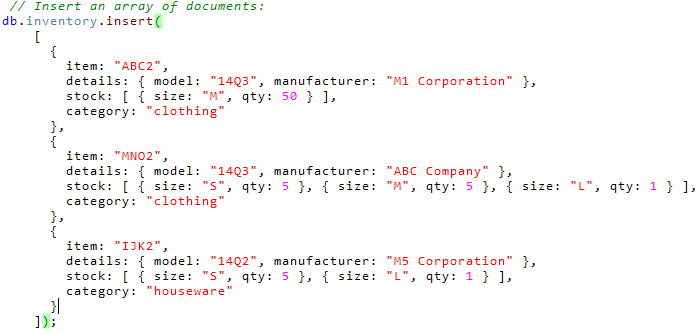
Additional Information: We can also insert an array of documents at once:

Note: This is an official MongoDB example taken from the documentation.

1.b) READ

In MongoDB, the db.collection.find() method retrieves documents from a collection. By default, the db.collection.find() method returns all the documents in a collection. This function has other uses as well which I plan to discuss later.

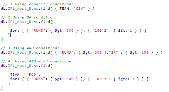
There are four types of READ operations as listed below:

1. Specifying an equality 
2. Using the OR
3. Using the AND
4. Using both OR & AND

These operations are described in the screenshot shown below:

Additional Information: How to perform querying on embedded documents?

Documents embedded within another document can be dealt with in the following two ways:

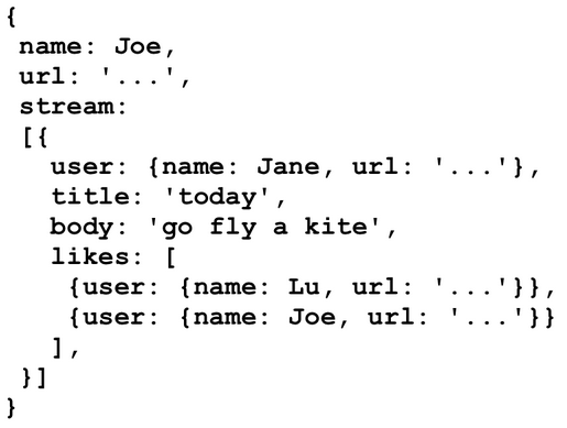
By now, people who are familiar with SQL must have realized the differences in syntax of MongoDB and SQL. Moreover,  the username.lastname  functionality shown above, is exclusive to NoSQL DBMS because of its embedded documents feature. It is also useful for extracting information from websites like Facebook as shown in the template below:

1. c) UPDATE

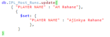
MongoDB provides update() method to update the documents of a collection. The method accepts the following parameters:

1. An update conditions document to match the documents to update.
2. An update operations document to specify the modification to perform, and
3. An options document.

The screenshot below shows the commands to use Update operation:

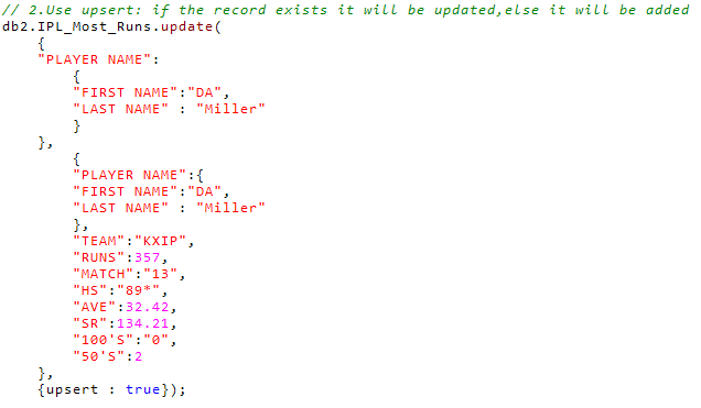
Use of UPSERT in UPDATE operation

The update() method will not give any output in case no document matches the condition query. However, if we specify upsert:true, update() will add a new document in case it doesn’t exist. If the doc exists upsert just does the update. Let’s see how!

1. d) REMOVE

In MongoDB, the db.collection.remove() method removes documents from a collection. We can remove all documents from a collection by removing all documents that match a condition, or limiting the operation to remove just a single document. Let’s see how.

Note: In the last line of code, the value 1 specifies only a single document which matches the criteria must be removed.

1. e) Aggregation operations

The data records in MongoDB can be processed by various operations for aggregation. After processing, it returns the computed results. It collects values from multiple documents, clubs the values and performs a variety of operations on the grouped data to return a single result. MongoDB provides multiple ways to perform aggregation. I have explained two of them, namely: Aggregation Pipeline and Map-Reduce Function. 

Let’s see how to do it!

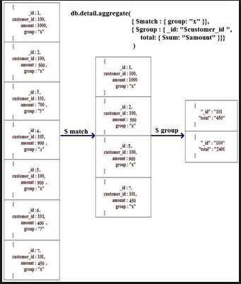
Aggregation Pipeline:

How does this aggregation pipeline works?

MongoDB aggregation pipelines consist of stage based transformation of data. All pipeline stages do not necessarily produce new documents. The stages might appear multiple times in the pipeline.

Infact, some stages might take pipeline expressions as operand, which specify the transformation to be done (ex: $and). Mostly, expressions are evaluated only when they are encountered in the pipeline but accumulates expressions such as $sum, $max. These expressions are then encountered during the $group stage is maintained throughout and the collective result is maintained till the pipeline code ends.

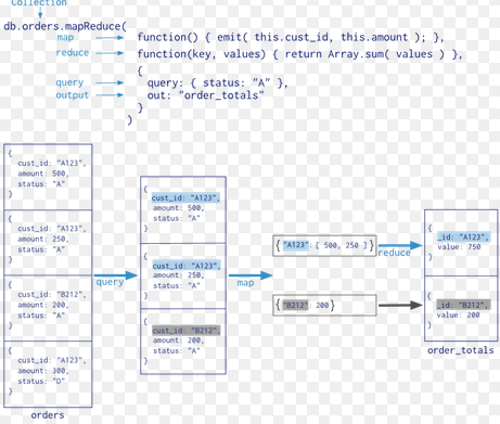
Map Reduce

How does Map Reduce operation works?

In the map-reduce operation, the map phase is applied to each input record which matches the query condition and key-value pairs are then emitted. For the keys that have multiple values, the reduce phase aggregates the collected data and finally the data is stored in a collection. Below is the visual representation of this operation:

Must Read:  Introduction to MapReduce

Codes for Aggregation and Map Reduce in MongoDB

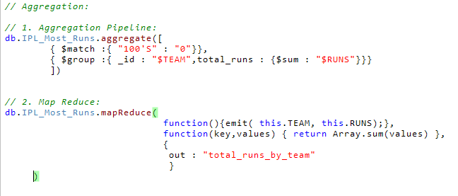
By this, we complete the overview of some basic operations in MongoDB.

Note: All the codes done here in the NoSQL manager can be done similarly in the Mongo Shell. I have used NoSQL here for ease of illustration.

2.1 Using RMongo Package

In the previous section, we got familiar with some basic coding in MongoDB. But as analysts, most of the work we do, will be done by using a statistical software. We connect the tool of our choice to the database, extract data to generate useful insights.

In this section, we will see how to use a package called RMongoDB which provides an interface to the NoSQL MongoDB database using the MongoDB C-driver version 0.8. – source: CRAN.

So, let’s quickly begin by installing the package. Use the codes below to install this package.

install.packages("Rmongo")
library(Rmongo) 
                                    

The dataset ‘output_rcb’ which contains only the documents of RCB is shown above. We’ll now use this dataset to explain operations using MongoDB.

An advantage of using RMongo package is that, its syntax is similar to MongoDB shell. Hence, operations like record, insertion, deletion can be performed in the similar fashion.

Also Read: The list of best resources to learn R Programming

Aggregation

Performing aggregation in Rmongo package is similar to performing it in MongoDB.

output_aggr <- dbAggregate(mongo,"IPL_Most_Runs",
                            c(' { "$match" : { "AVE" : {"$gt" : 40}}} ',
                            ' { "$group" : { "_id" : "$TEAM","total_Runs" : { "$sum" : $RUNS" }}} ))

Here, our motive is to match records from the IPL_Most_Runs collection where the Average is more than 40. Then, we’ll group those records by team and sum up the Runs within each group. Let’s see how can we do it.

[1] "{ \"_id\" : \"DD\" , \"total_Runs\" : 414.0}"   "{ \"_id\" : \"RCB\" , \"total_Runs\" : 1509.0}"
[3] "{ \"_id\" : \"MI\" , \"total_Runs\" : 540.0}"   "{ \"_id\" : \"RR\" , \"total_Runs\" : 540.0}"
[5] "{ \"_id\" : \"SRH\" , \"total_Runs\" : 562.0}"

We can see that the output is not a dataframe. This is a common problem faced when using these R packages to interact with MongoDB. Since MongoDB stores data internally as BSON, converting them into data frames and performing complex queries such as aggregation, fails to store the results in a data frame except when the data is of primitive type. But simpler queries like dbGetQuery results in a dataframe.

A drawback of using this package is, you cannot use it with MapReduce.

2.2 Using Mongolite Package

We got familiar with the use of RMongo package and few of its limitation also. There is another package in R called ‘Mongolite’ which provides another way to connect to a MongoDB instance. This package has been recently released on 12^th May, 2015. Hence, not many people have started using it.

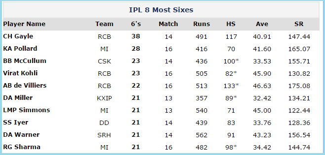
We will use the dataset shown below for illustrations:

Connect to a MongoDB instance

After installing and loading the package into R library, we need to establish a connection to a MongoDB instance and a database in it.

m <- mongo(collection = "IPL_Most_Sixes",db = "test",url = "mongodb://localhost")

This creates a collection called IPL_Most_Sixes in the database “test”.

Insert

For this package we have to load a dataframe into R and then insert it into the MongoDB instance. After importing the data into R we insert it into the IPL_Most_Sixes collection created above.

sixes <- read.csv("C:/Users/DELL/Desktop/IPL_Most_Sixes.csv",sep = ",",header = T)
m$insert(sixes)

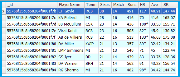
Let’s view the data in the collection:

Return only chosen fields

rcb = m$find('{"Team": "RCB"}','{"PlayerName" : 1,"Sixes" : 1,"SR" : 1,"_id" : 0}')

This returns only the fields PlayerName, Sixes and SR for the records where the Team is “RCB”. The result is a data frame object.

We can also update and remove entries from the database. But, the commands for those operations are similar to what we have already seen in this article, here we are going to look at Aggregation and Map-Reduce in the mongolite package.

Aggregation

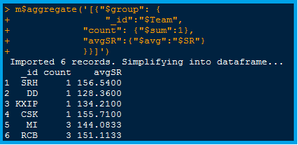
We can do aggregation similar to the previous sections using the aggregate function in this package.

As. it can be seen, only the required fields are loaded from MongoDB and it will results in considerable performance enhancement in case of large data sets. Also, the result has been internally converted to a data frame.

MapReduce

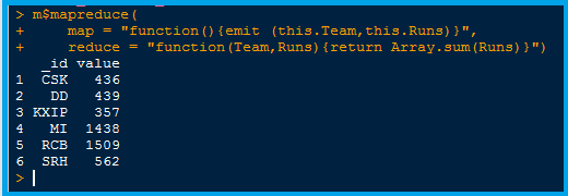The map and reduce functions calculate the sum of runs grouped by teams.These results can be stored in a data frame in R for further analysis as shown above.

Hence, these two packages (RMongo & Mongolite) in R can be used to deal with data from MongoDB albeit some limitations. There is another package called “rmongodb” which can be used.

However, the results generated from data manipulation using rmongodb are JSON objects and are not very useful. The syntax is also very complex compared to the other two packages.

Till now, we have learnt how to access MongoDB from R . Let’s move into Python and see what libraries are there to deal with similar cases.

Also Read: Best ways to perform data manipulation using MapReduce

3. Using PyMongo

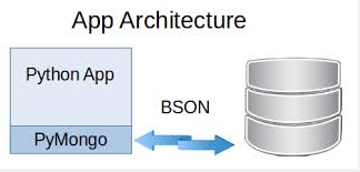
PyMongo is a Python distribution containing tools for working with MongoDB, and is the recommended way to work with MongoDB from Python.

import pymongo
from pymongo import MongoClient
client = MongoClient('localhost', 27017)

We will be using the dataset shown below:

We will create a collection called pymongo and perform operations using the pymongo library.

Insert records

• Insert single records

The command db.pymongo creates the database pymongo if it does not exist. Here we’ll insert only one record. As you can see the Stats column is an embedded document in itself.

• Bulk Insert

We have inserted 5 records in total into the collection called pymongo. Lets view it in NoSQL manager

Querying one or more than one document

The find_one() is used to find a single document in a collection. If we do not pass any arguments to it,the first document will be returned. If we pass any condition, in that case, the first document matching the condition is returned.

For querying multiple documents, a for loop is used as shown in the image above. Here, we want to see only those records where the number of ducks are <= 2.

Notice the Stats.Ducks part, this is the syntax to be used when we want to query within embedded documents.

Also Read: A Quick Guide to learn Python for Data Science

Aggregation 

In this section we will see how to perform aggregation in Pymongo using Pipelines and Map Reduce.

1.Using Pipeline

The unwind command opens up the embedded document Stats for further manipulation. Here we are trying to calculate how many ducks are there for each value of duck. For example, there are 4 records having 2 ducks each, hence a total of 8 ducks.

2. Using Map Reduce

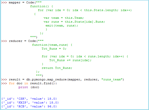
The mapper function creates an array of runs for each team and the reducer function sums the runs grouped by each team. The results are stored in the collection runs_team.

4.1 Using JSON Studio for accessing MongoDB

Aggregations is one of the strong points of the MongoDB framework and can be done quite easily in Mongo Shell, R & Python. There is another package in R called jSonarR: jSonar Analytics Platform API for R

“This package enables users to access MongoDB by running queries and returning their results in R data frames. Usually, data in MongoDB is only available in the form of a JSON document. jSonarR uses data processing and conversion capabilities in the jSonar Analytics Platform and the JSON Studio Gateway , to convert it to a tabular format which is easy to use with existing R packages.”- Source : CRAN-jSonarR

Before we dig into the jSonarR package, let’s get a basic understanding of using JSON Studio for interfacing with MongoDB. We will take a look at :

• Creating an aggregation pipeline.
• Basic Visualisations.
• Writing and executing code.

Here is the Installation Guide for JSON Studio.

Once you’ve installed JSON Studio, perform the following operations.

Creating an Aggregation Pipeline:

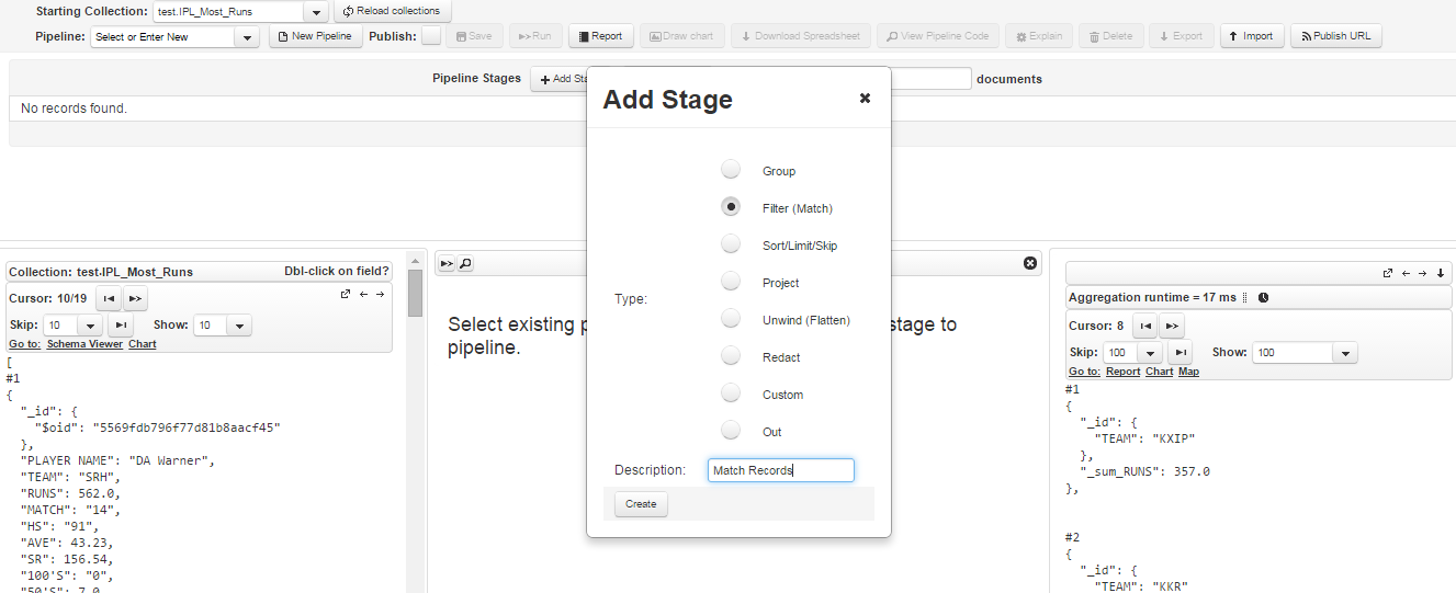
1. Click on New pipeline.
2. Click on Add Stage and select the operation for the first stage. If you want a match to be performed at first and then grouping on the matched data, select Filter(Match) as shown below:

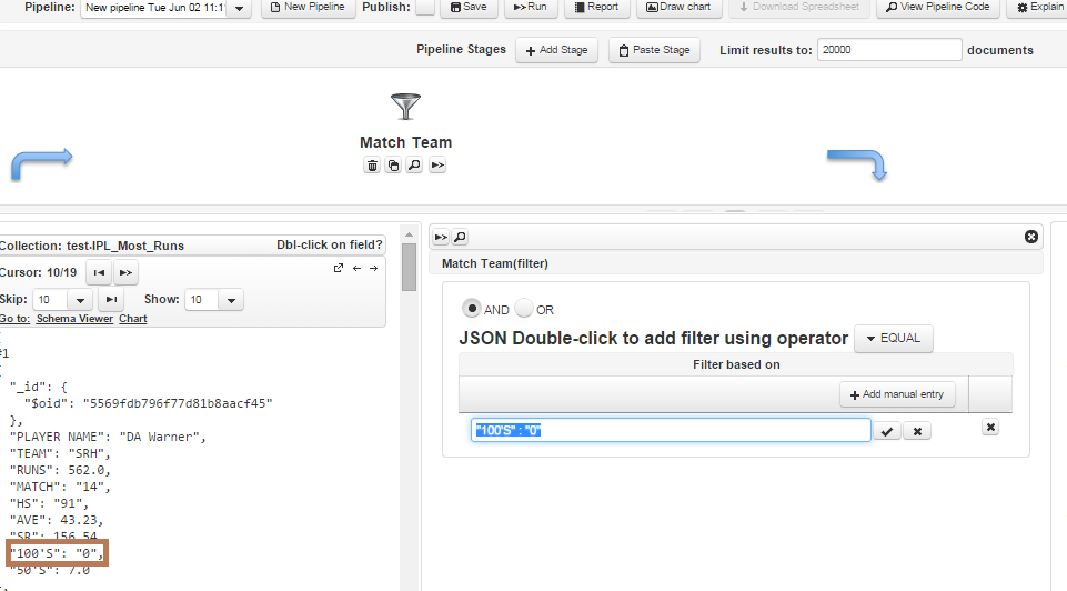
3. After the first stage is created, we need to define the variables for the stage (Match Records in our case). We want the matching to be done on records where the value of 100’s is “0”, so this has to be entered in the box that opens after clicking on 100’s on the LHS (marked in brown box) as shown below:

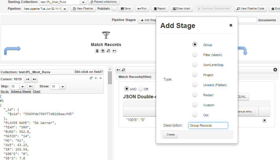
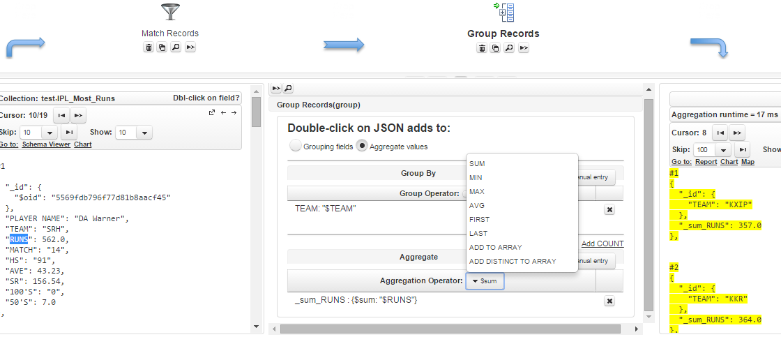
4. Now we’ll create a second stage aggregation called Group Records that will group the records by team and calculate the total runs by team.

5. After creating the second stage, we’ll define the grouping fields and aggregate fields by clicking on the respective fields on LHS. For aggregation, we need to define the aggregate function from the drop-down which appears when we click on Aggregation Operator below Aggregate as shown below:

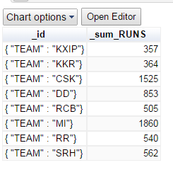
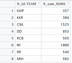
6. Click on Save and then Run. Once the pipeline has been run the results can be viewed by clicking on the Report on the right hand bottom side. This opens up a new window that contains the results in a tabular form. In our case they are:

You can also see the code for  pipeline by clicking on View Pipeline Code. You can save the pipeline for future use as well. There is also a chart option which can be used to visualize the output of the aggregation.

Below are the illustrations of output of aggregation using basic visualization methods. Let’s look at the steps to create them:

Basic Visualizations

1. Load the collections in a database and then click on any one of them.Then click on execute.
2. After the collection is displayed click on Draw Chart.
3. Choose from options to draw the desired visualization.

Note: At times, all the documents in a collection might not be loaded into the chart window. In that case, click on + to bring in all the documents.

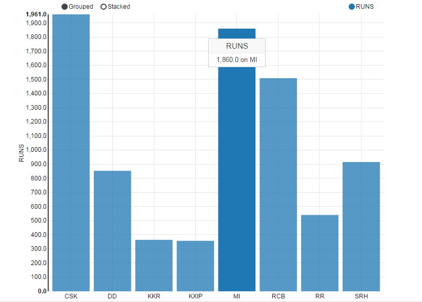
As you can see above, the bar chart has been created from IPL_Most_Runs data. It is also an interactive chart, RUNS of MI are displayed when we hover above the bar for MI as shown above.

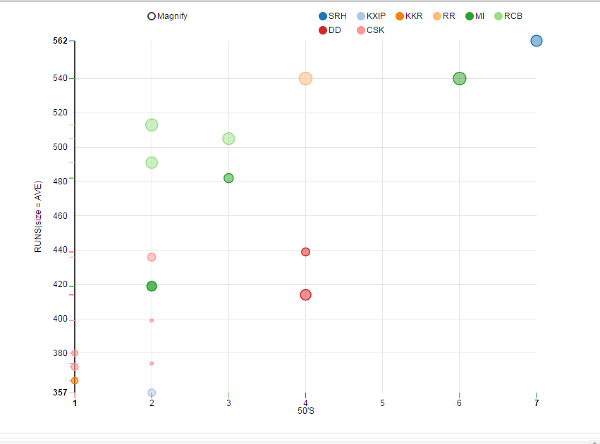
Here is another chart:

Here the distribution of runs scored by the number of 50’s scored is displayed on a scatter plot. The size of the bubble is according to the average of the particular batsman and the grouping has been done on team.

Writing and executing Code for visualizations

We can also execute code in JSON studio. If you have grasped the syntax of MongoDB shown in the first part ,executing code here will not be an issue.

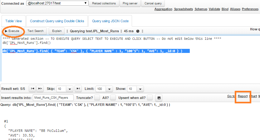
The code basically remains the same but only db.IPL_Most_Runs.find() is replaced by db[‘IPL_Most_Runs’].find() as shown below:

Select the highlighted portion and click on Execute. The results are JSON objects which get displayed in the results window. You can click on Report to see a tabular format of the output. The results can also be saved into another collection by using the Insert results into: option.

These were some of the basic operations that can be done using JSON studio.Though modeling techniques such as regression,clustering etc. cannot be applied using JSON it is definitely a great tool for exploring data, especially when using unstructured data gleaned from MongoDB.

4.2. Using jSonarR

Now that we have an understanding of how JSON studio functions, lets quickly take a look at the “jSonarR” package.

Illustration

Lets see how we can use the aggregation pipeline we had created in the preceding section to load the resultant data into R and view it as a data frame.

1. After starting the MongoDB session, start Json Studio.
2. Now login is established, connect to the database where the collections are stored
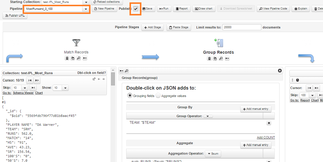
3. Then, click on aggregation.

4. After the page shown above loads completely,  we can see the name of our aggregation pipeline and a Publish option.
5. Click on Publish so that an API is published to which R can connect and retrieve data through it.
6. Then run the following code in R:

connection <- new.SonarConnection('https://dell-pc:8443', 'localhost', 'test')

aggr <- sonarAgg(connection, 'MostRunsand_0_100', 'IPL_Most_Runs')

7. The https://dell-pc:8443 is the url through which Json Studio runs in the system. It will be displayed in the url bar when you start Json Studio. It varies from system to system.
8. The sonarAgg function is used to load the results of an aggregation into R.

Now lets see the structure of the data loaded.

We can see that the data has been loaded as a data frame in R. With this data frame, we can do any further analysis as we might want to.

Note:

All the data has been compiled from IPL Statistics.

If you wish to learn more about Json Studio, please visit : http://jsonstudio.com/

If you wish to learn more about jSonarR package in R, please visit jSonarR.

End Notes

A comprehensive knowledge of databases is not required by an analyst, but knowing how to access a database and getting data into the local environment for further use is certainly beneficial.

In this article, we learnt how to deal with MongoDB data using R,Python and Json Studio. This was not aimed at providing the reader with a comprehensive knowledge of any one method but rather as a quick guide to several methods. Choose the one as per your need and comfort.!!

I hope this article helped you to get acquainted with basics of MongoDB packages. We would love to hear about it from you. Did you find it useful? Feel free to post your thoughts through comments below.

If you like what you just read & want to continue your analytics learning, subscribe to our emails, follow us on twitter or like our facebook page.