Beginners Guide to Content Based Recommender Systems

One of the most surprising part about Content Based Recommender Systems is, ‘we summon to its suggestions / advice every other day, without even realizing that’. Confused? Let me show you some examples. Facebook, YouTube, LinkedIn are among the most used websites on Internet today. Let us see how they use recommender systems. You’ll be amazed!

Facebook: Suggests us to make more friends using ‘People You May Know’ section

Similarly LinkedIn suggests you to connect with people you may know and YouTube suggests you relevant videos based on your previous browsing history. All of these are recommender systems in action.

While most people know about these features, only a few understand that experts call the algorithms behind them ‘Recommender Systems’. They ‘recommend’ personalized content on the basis of user’s past / current preference to improve the user experience. Broadly, there are two types of recommendation systems – Content Based & Collaborative filtering based. In this article, we’ll learn about content based recommendation system.

But before we proceed, let me define a couple of terms:

• Item would refer to content whose attributes are used in the recommender models. These could be movies, documents, book etc.
• Attribute refers to the characteristic of an item. A movie tag, words in a document are examples.

What are Content Based Recommender Systems?

Content-based recommender systems are a subset of recommender systems that tailor recommendations to users by analyzing items’ intrinsic characteristics and attributes. These systems focus on understanding the content of items and mapping it to users’ preferences. By examining features such as genre, keywords, metadata, and other descriptive elements, content-based recommender systems create profiles for both users and items.

This enables the system to make recommendations matching user preferences with items with similar content traits. Unlike collaborative filtering methods that depend on historical interactions among users, content-based systems operate independently, which makes them particularly useful in scenarios where user history is limited or unavailable. Through this personalized approach, content-based recommender systems play a vital role in enhancing user experiences across various domains, from suggesting movies and articles to guiding users in choosing products or destinations.

Also Read: Information Retrieval System explained in simple terms!

How Do Content Based Recommender Systems Work?

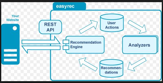
A content based recommender works with data that the user provides, either explicitly (rating) or implicitly (clicking on a link). Based on that data, a user profile is generated, which is then used to make suggestions to the user. As the user provides more inputs or takes actions on the recommendations, the engine becomes more and more accurate.

Image Source: easyrec.org

What are the concepts used in Content Based Recommenders?

The concepts of Term Frequency (TF) and Inverse Document Frequency (IDF) play a crucial role in information retrieval systems and content-based filtering mechanisms, such as content-based recommenders. These concepts help determine the relative importance of a document, article, news item, movie, etc.

Term Frequency (TF) and Inverse Document Frequency (IDF)

TF is simply the frequency of a word in a document. IDF is the inverse of the document frequency among the whole corpus of documents. TF-IDF is used mainly because of two reasons: Suppose we search for “the rise of analytics” on Google. It is certain that “the” will occur more frequently than “analytics” but the relative importance of analytics is higher than the search query point of view. In such cases, TF-IDF weighting negates the effect of high frequency words in determining the importance of an item (document).

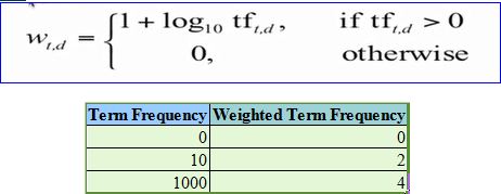
But while calculating TF-IDF, log is used to dampen the effect of high frequency words. For example: TF = 3 vs TF = 4 is vastly different from TF = 10 vs TF = 1000. In other words the relevance of a word in a document cannot be measured as a simple raw count and hence the equation below:

Equation:

You can observe that high-frequency words have a dampened effect, making these values more comparable to each other than the original raw term frequency.

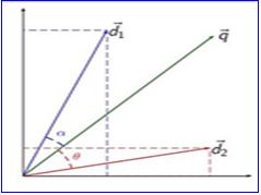
After calculating TF-IDF scores, how do we determine which items are closer to each other, rather closer to the user profile? You accomplish this using the Vector Space Model, which computes proximity based on the angle between the vectors.

How does Vector Space Model Works?

In this model, you store each item as a vector of its attributes (which are also vectors) in an n-dimensional space and calculate the angles between the vectors to determine the similarity. Next, you create user profile vectors based on their actions on previous attributes of items, and you determine the similarity between an item and a user in a similar way.

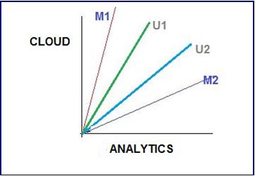
Lets try to understand this with an example.

Shown above is a 2-D representation of a two attributes, Cloud & Analytics. M1 & M2 are documents. U1 & U2 are users. The document M2 is more about Analytics than cloud whereas M1 is more about cloud than Analytics. I am sure you want to know how the relative importance of documents are measures. Hold on, we are coming to that.

User U1, likes articles on the topic ‘cloud’ more than the ones on ‘analytics’ and vice-versa for user U2. You calculate the user’s likes, dislikes, and measures by taking the cosine of the angle between the user profile vector (Ui) and the document vector.

The ultimate reason behind using cosine is that the value of cosine will increase with decreasing value of the angle between which signifies more similarity. You length-normalize the vectors, which then become vectors of length 1, and the cosine calculation simply involves the sum-product of the vectors. We will be using the function sumproduct in excel which does the same to calculate similarities between vectors in the next section.

Case Study 1: How to Calculate TF – IDF ?

Let’s understand this with an example. Suppose, we search for “IoT and analytics” on Google and the top 5 links that appear have some frequency count of certain words as shown below:

Among the corpus of documents and blogs used to search for articles, 5,000 documents contain the word “analytics,” 50,000 contain “data,” and other words have similar counts. Let us assume that the total corpus of docs is 1 million(10^6).

Term Frequency (TF)

As seen in the image above, for article 1, the term Analytics has a TF of 1+ log₁₀21 = 2.322. In this way, TF is calculated for other attributes of each of the articles. These values make up the attribute vector for each of the articles.

Inverse Document Frequency (IDF)

You calculate IDF by taking the logarithmic inverse of the document frequency across the entire corpus of documents. For example, if a total of 1 million documents return from our search query and ‘smart’ appears in 0.5 million of those documents, you can determine its IDF. Thus, it’s IDF score will be: Log₁₀ (10^6/500000) = 0.30.

You can see in the image above that the most commonly occurring term ‘smart‘ receives the lowest weight from IDF. You calculate the length of these vectors as the square root of the sum of the squared values of each attribute in the vector:

After we have found out the TF -IDF weights and also vector lengths, let’s normalize the vectors.

Each term vector is divided by the document vector length to get the normalized vector. So, for the term ‘Analytics’ in Article 1, the normalized vector is: 2.322/3.800. Similarly, normalize all the terms in the document, and as you can see in the image above, each document vector now has a length of 1.

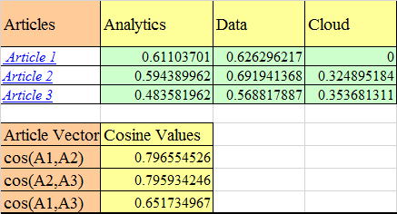
Now, that we have obtained the normalized vectors, let’s calculate the cosine values to find out the similarity between articles. For this purpose, we will take only three articles and three attributes.

Cos(A1,A2) is simply the sum of dot product of normalized term vectors from both the articles. The calculation is as follows:

Cos(A1,A2) = 0.611*0.59 + 0.63 * 0.69 + 0* 0.32 = =.7965

As you can see the articles 1 and 2 are most similar and hence appear at the top two positions of search results. Also, if you remember we had said that Article 1 (M1) is more about analytics than cloud-Analytics has a weight of 0.611 whereas cloud has 0 after length normalization.

Case Study 2: Creating Binary Representation

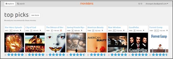
This picture is an example of movie recommender system called movielens. This is a movie recommendation site which recommends movies you should watch based on which movies you have rated and how much you have rated them.

At a rudimentary level, the system takes in my inputs and creates a profile based on the attributes that reflect my likes and dislikes (which may be based on some keywords or movie tags I have liked or ignored).

I have liked 52 movies across various genres. These items (movies) are attributes since it can help us to determine a user’s taste. Below is the list of the top 6 movies recommended by MovieLens. The user columns specify whether a user has liked / disliked a recommended movie. The 1/0 simply represent whether the movie has adventure/action etc. or not. You call this type of representation a binary representation of attributes.

In the above example, user 1 has liked Star Wars whereas user 2 has not. Based on these types of inputs a user profile is generated.

Other metrics like count data, simple 1 / 0 representation are also used. The measure depends upon the context of use. For example: for normal movie recommender system, a simple binary representation is more useful whereas for a search query in search engine like google, a count representation might be more appropriate.

Building a Content Based Recommender for Analytics Vidhya (AV)

Now that we have learned all these concepts, let’s actually try to build a simple content based recommender based on user taste for AV. Many articles have been published on AV. Every article published caters to  a segment of audience such that some people might like articles on machine learning algorithms, while other might like R over machine learning. Hence, having a recommender system would help.

To build the recommender system:

Step 1

In each week, for each user, we will track user engagement (like / share / comments) with various articles. Let’s see how that can be done:

We have used binary representation here. The image shown above represents, Article 1 is about big data, python and learning path. Similarly, article 2 is about R, python and machine learning. User 1 has liked article 1 (shared it on social media) and has not liked article 2. You have not engaged with articles 3, 4, and 5 except for reading them.

Step 2: Normalize

For binary representation, we can perform normalization by dividing the term occurrence(1/0) by the sqrt of number of attributes in the article. Hence, for Article 1: normalized attribute = 1/sqrt(3) = 0.577.

A question that you must ask here is: what happened to TF? and why did we directly do normalization before calculating the TF scores? If you calculate TF without normalization, the TF scores will be 1+log ₁₀ 1 = 1 for attributes that occur and simply 0 for attributes that don’t. And, thus the TF scores will also becomes 1/0.

Step 3: User Profile

Let’s see how the user profiles are generated by using the ‘sumproduct’ function in excel.

You multiply each attribute column (see the highlighted learning paths columns above) with each user attribute value (highlighted part of User 2). This is simply the dot product of vectors that we saw earlier. This gives a user profile (as shown in the User Profiles part above) an understanding of user’s taste.

Thus, user 1 likes articles on big data most(highest score of 1.28) followed by learning paths and then machine learning. Similarly, user 2 like articles on machine learning the most.

Now we have the user profile vectors and the article vectors, let’s use these to predict which articles will be similar to the user’s taste.

Note : The SUMPRODUCT function in the image above contains some vectors which are highlighted in the image. B36:F36 is the article 6 vector.

The dot product of article vectors and IDF vectors gives the weighted scores of each article. You then use these weighted scores for a dot product with the user profile vector (user 1 here). This gives a probability that the user will like a particular article. For article 1, the probability is 75%.

This concept can be applied to ‘n’ articles to determine which article a user will like the most. Therefore, along with new articles released in a week, you can make a separate recommendation to a particular user based on the articles they haven’t read yet.

Limitations of Content Based Recommender Systems

Content based recommenders have their own limitations. They are not good at capturing inter-dependencies or complex behaviors. For example: I might like articles on Machine Learning, only when they include practical application along with the theory, and not just theory. This type of information cannot these recommenders capture.

Conclusion

In this article, we have seen two approaches to content based recommenders. They both use the TF-IDF weighting and vector space model implementations, albeit in different ways. So While the count data helped us understand the methodology for calculating the weighted scores of articles, the binary representation clarified how to calculate scores for data represented as 1/0. We also saw how user profiles generate and how predictions rely on that information.

I have intentionally left the column PredUser2 empty in case you would like to go ahead and calculate it.

Did you find this article useful ? Have you also worked on recommender systems? Share your opinions / views in the comments section below.

Frequently Asked Questions