Do Faster Data Manipulation using These 7 R Packages

Introduction

Data Manipulation is an inevitable phase of predictive modeling. A robust predictive model can’t just be built using machine learning algorithms. But, with an approach to understand the business problem, the underlying data, performing required data manipulations and then extracting business insights.

Among these several phases of model building, most of the time is usually spent in understanding underlying data and performing required manipulations. This would also be the focus of this article – packages to perform faster data manipulation in R.

What is Data Manipulation ?

If you are still confused with this ‘term’, let me explain it to you. Data Manipulation is a loosely used term with ‘Data Exploration’. It involves ‘manipulating’ data using available set of variables. This is done to enhance accuracy and precision associated with data.

Actually, the data collection process can have many loopholes. There are various uncontrollable factors which lead to inaccuracy in data such as mental situation of respondents, personal biases, difference / error in readings of machines etc. To mitigate these inaccuracies, data manipulation is done to increase the possible (highest) accuracy in data.

At times, this stage is also known as data wrangling or data cleaning.

Different Ways to Manipulate / Treat Data:

There is no right or wrong way in manipulating data, as long as you understand the data and have taken the necessary actions by the end of the exercise. However, here are a few broad ways in which people try and approach data manipulation. Here are they:

• Usually, beginners on R find themselves comfortable manipulating data using inbuilt base R functions. This is a  good first step, but is often repetitive and time consuming.  Hence, it is a less efficient way to solve the problem.
• Use of packages for data manipulation. CRAN has more than 7000 packages available today. In simple words, these packages are nothing but a collection of pre-written commonly used pieces of codes. They help you perform the repetitive tasks fasts, reduce errors in coding and take help of code written by experts (across the open source eco-system for R) to make your code more efficient. This is usually the most common way of performing data manipulation.
• Use of ML algorithms for data manipulation. You can use tree based boosting algorithms to take care of missing data & outliers. While these are definitely less time consuming, these approaches typically leave you wanting for a better understanding of data at the end of it.

Hence, more often than not, use of packages is the de-facto method to perform data manipulation. In this article, I have explained several packages which make ‘R’ life easier during the data manipulation stage.

Note: This article is best suited for beginners in R Language. You can install a packages using:

install.packages('package name')

List of Packages

For better understanding, I’ve also demonstrated their usage by undertaking commonly used operations. Below is the list of packages discussed in this article:

1. dplyr
2. data.table
3. ggplot2
4. reshape2
5. readr
6. tidyr
7. lubridate

Note: I understand ggplot2 is a graphical package. But, it generally helps in visualizing data ( distributions, correlations) and making manipulations accordingly. Hence, I’ve added it in this list. In all packages, I’ve covered only the most commonly used commands in data manipulation.

dplyr Package

This packages is created and maintained by Hadley Wickham. This package has everything (almost) to accelerate your data manipulation efforts. It is known best for data exploration and transformation. It’s chaining syntax makes it highly adaptive to use. It includes 5 major data manipulation commands:

1. filter – It filters the data based on a condition
2. select – It is used to select columns of interest from a data set
3. arrange – It is used to arrange data set values on ascending or descending order
4. mutate – It is used to create new variables from existing variables
5. summarise (with group_by) – It is used to perform analysis by commonly used operations such as min, max, mean count etc

Simple focus on these commands and do great in data exploration. Let’s understand these commands one by one. I have used 2 pre-installed R data sets namely mtcars and iris.

> library(dplyr)
> data("mtcars")
> data('iris')

> mydata <- mtcars

#read data
> head(mydata)

#creating a local dataframe. Local data frame are easier to read

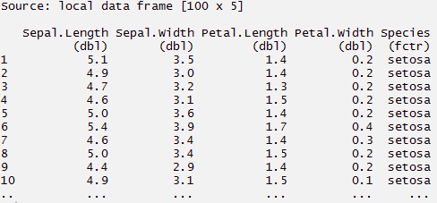
> mynewdata <- tbl_df(mydata)
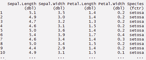
> myirisdata <- tbl_df(iris)

#now data will be in tabular structure
> mynewdata



> myirisdata

#use filter to filter data with required condition
> filter(mynewdata, cyl > 4 & gear > 4 )



> filter(mynewdata, cyl > 4)



> filter(myirisdata, Species %in% c('setosa', 'virginica'))

#use select to pick columns by name
> select(mynewdata, cyl,mpg,hp)



#here you can use (-) to hide columns
> select(mynewdata, -cyl, -mpg ) 


#hide a range of columns
> select(mynewdata, -c(cyl,mpg))

#select series of columns

> select(mynewdata, cyl:gear)

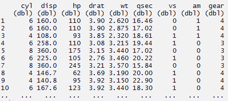
#chaining or pipelining - a way to perform multiple operations
#in one line
> mynewdata %>%
     select(cyl, wt, gear)%>%
     filter(wt > 2)

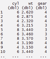
#arrange can be used to reorder rows
> mynewdata%>%
     select(cyl, wt, gear)%>%
     arrange(wt)

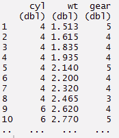
#or

> mynewdata%>%
     select(cyl, wt, gear)%>%
     arrange(desc(wt))

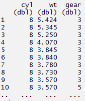
#mutate - create new variables

> mynewdata %>%
      select(mpg, cyl)%>%
      mutate(newvariable = mpg*cyl)

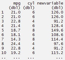
#or

> newvariable <- mynewdata %>% mutate(newvariable = mpg*cyl)

#summarise - this is used to find insights from data
> myirisdata%>%
       group_by(Species)%>%
       summarise(Average = mean(Sepal.Length, na.rm = TRUE))

#or use summarise each

> myirisdata%>%
      group_by(Species)%>%
      summarise_each(funs(mean, n()), Sepal.Length, Sepal.Width)



#You can create complex chain commands using these 5 verbs.

#you can rename the variables using rename command
> mynewdata %>% rename(miles = mpg)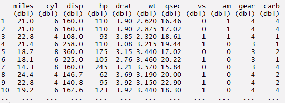

data.table Package

This package allows you to perform faster manipulation in a data set. Leave your traditional ways of sub setting rows and columns and use this package. With minimum coding, you can do much more. Using data.table helps in reducing computing time as compared to data.frame. You’ll be astonished by the simplicity of this package.

A data table has 3 parts namely DT[i,j,by]. You can understand this as, we can tell R to subset the rows using ‘i’, to calculate ‘j’ which is grouped by ‘by’. Most of the times, ‘by’ relates to categorical variable. In the code below, I’ve used 2 data sets (airquality and iris).

#load data
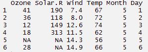
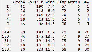
> data("airquality")
> mydata <- airquality
> head(airquality,6)

> data(iris)
> myiris <- iris

#load package
> library(data.table)

> mydata <- data.table(mydata)
> mydata

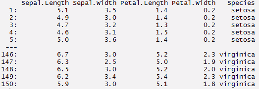
> myiris <- data.table(myiris)
> myiris

#subset rows - select 2nd to 4th row

> mydata[2:4,]

#select columns with particular values
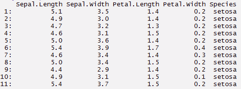
> myiris[Species == 'setosa']

#select columns with multiple values. This will give you columns with Setosa
#and virginica species
> myiris[Species %in% c('setosa', 'virginica')]

#select columns. Returns a vector
> mydata[,Temp]

> mydata[,.(Temp,Month)]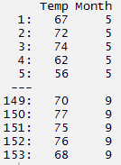

#returns sum of selected column
> mydata[,sum(Ozone, na.rm = TRUE)]

[1]4887

#returns sum and standard deviation
> mydata[,.(sum(Ozone, na.rm = TRUE), sd(Ozone, na.rm = TRUE))]

#print and plot
> myiris[,{print(Sepal.Length)
> plot(Sepal.Width)
 NULL}]

#grouping by a variable
> myiris[,.(sepalsum = sum(Sepal.Length)), by=Species]

#select a column for computation, hence need to set the key on column
> setkey(myiris, Species)

#selects all the rows associated with this data point
> myiris['setosa']
> myiris[c('setosa', 'virginica')]

ggplot2 Package

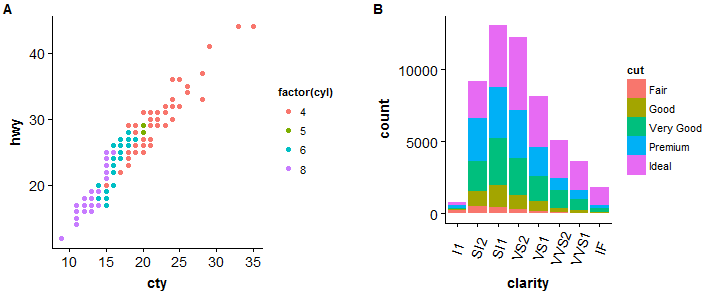
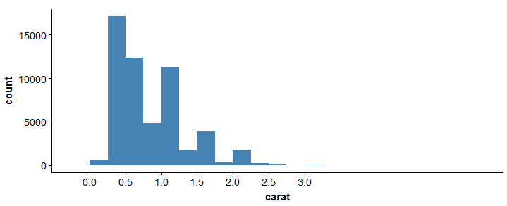
ggplot offers a whole new world of colors and patterns. If you are a creative soul, you would love this package till depth. But, if you wish learn what is necessary to get started, follow the codes below. You must learn the ways to at least plot these 3 graphs: Scatter Plot, Bar Plot, Histogram.

These 3 chart patterns covers almost every type of data representation except maps. ggplot is enriched with customized features to make your visualization better and better. It becomes even more powerful when grouped with other packages like cowplot, gridExtra. In fact, there are a lot of features. Hence, you must focus on few commands and build your expertise on them. I have also shown the method to compare graphs in one window. It requires ‘gridExtra’ package. Hence, you must install it. I’ve use pre-installed R data sets.

> library(ggplot2)
> library(gridExtra)
> df <- ToothGrowth

> df$dose <- as.factor(df$dose)
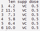
> head(df)

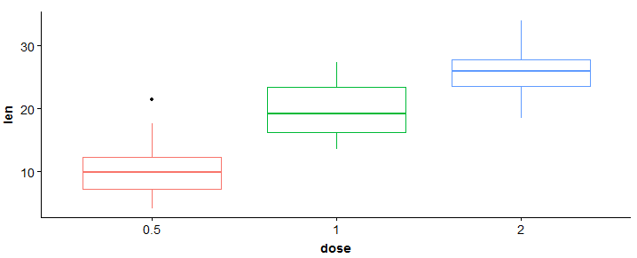
#boxplot
> bp <- ggplot(df, aes(x = dose, y = len, color = dose)) + geom_boxplot() + theme(legend.position = 'none')
> bp

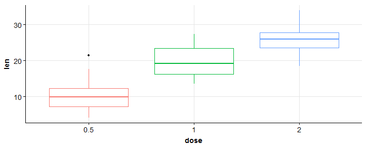
#add gridlines
> bp + background_grid(major = "xy", minor = 'none')

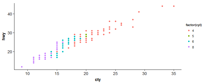
#scatterplot
> sp <- ggplot(mpg, aes(x = cty, y = hwy, color = factor(cyl)))+geom_point(size = 2.5)
> sp

#barplot
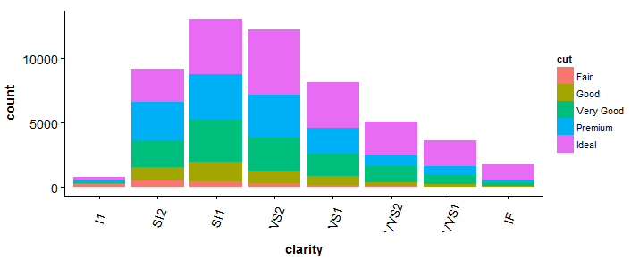
> bp <- ggplot(diamonds, aes(clarity, fill = cut)) + geom_bar() +theme(axis.text.x = element_text(angle = 70, vjust = 0.5))
> bp

#compare two plots
> plot_grid(sp, bp, labels = c("A","B"), ncol = 2, nrow = 1)



#histogram
> ggplot(diamonds, aes(x = carat)) + geom_histogram(binwidth = 0.25, fill = 'steelblue')+scale_x_continuous(breaks=seq(0,3, by=0.5))

For more information on this package, you refer to cheatsheet here: ggplot2 cheatsheet

reshape2 Package

As the name suggests, this package is useful in reshaping data. We all know the data come in many forms. Hence, we are required to tame it according to our need. Usually, the process of reshaping data in R is tedious and worrisome. R base functions consist of ‘Aggregation’ option using which data can be reduced and rearranged into smaller forms, but with reduction in amount of information. Aggregation includes tapply, by and aggregate base functions. The reshape package overcome these problems. Here we try to combine features which have unique values. It has 2 functions namely melt and cast.

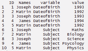
melt : This function converts data from wide format to long format. It’s a form of restructuring where multiple categorical columns are ‘melted’ into unique rows. Let’s understand it using the code below.

#create a data
> ID <- c(1,2,3,4,5)
> Names <- c('Joseph','Matrin','Joseph','James','Matrin')
> DateofBirth <- c(1993,1992,1993,1994,1992)
> Subject<- c('Maths','Biology','Science','Psycology','Physics')

> thisdata <- data.frame(ID, Names, DateofBirth, Subject)
> data.table(thisdata)

#load package
> install.packages('reshape2')
> library(reshape2)

#melt 
> mt <- melt(thisdata, id=(c('ID','Names')))
> mt

cast : This function converts data from long format to wide format. It starts with melted data and reshapes into long format. It’s just the reverse of melt function. It has two functions namely, dcast and acast. dcast returns a data frame as output. acast returns a vector/matrix/array as the output. Let’s understand it using the code below.

#cast
> mcast <- dcast(mt, DateofBirth + Subject ~ variable)
> mcast

Note: While doing research work, I found this image which aptly describes reshape package.

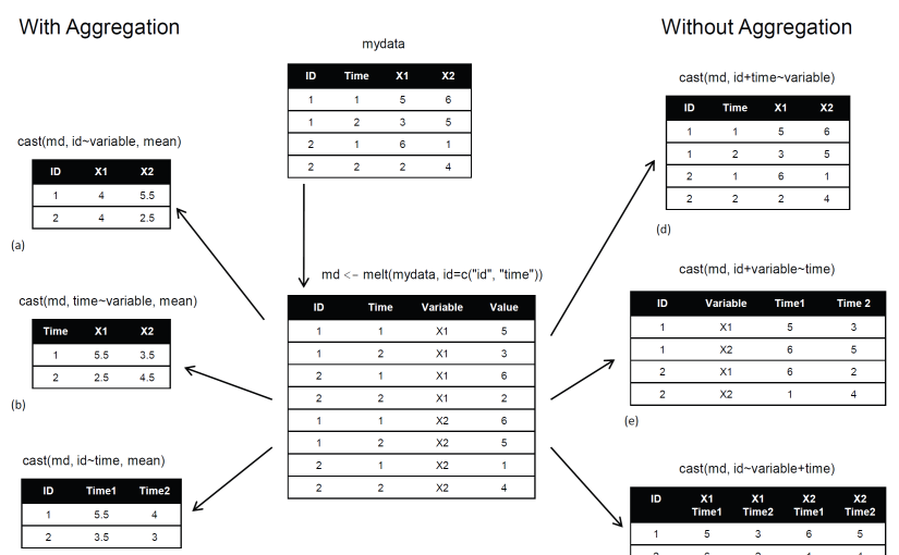                                                                                source: r-statistics

readr Package

As the name suggests, ‘readr’ helps in reading various forms of data into R. With 10x faster speed. Here, characters are never converted to factors(so no more stringAsFactors = FALSE). This package can replace the traditional read.csv() and read.table() base R functions. It helps in reading the following data:

• Delimited files withread_delim(), read_csv(), read_tsv(), andread_csv2().
• Fixed width files with read_fwf(), and read_table().
• Web log files with read_log()

If the data loading time is more than 5 seconds, this function will show you a progress bar too. You can suppress the progress bar by marking it as FALSE. Let’s look at the code below:

> install.packages('readr')
> library(readr)

> read_csv('test.csv',col_names = TRUE)

You can also specify the data type of every column loaded in data using the code below:

> read_csv("iris.csv", col_types = list(
      Sepal.Length = col_double(),
      Sepal.Width = col_double(),
      Petal.Length = col_double(),
      Petal.Width = col_double(),
      Species = col_factor(c("setosa", "versicolor", "virginica"))
))

However, if you choose to omit unimportant columns, it will take care of it automatically. So, the code above can also be re-written as:

> read_csv("iris.csv", col_types = list(
           Species = col_factor(c("setosa", "versicolor", "virginica"))
)

P.S – readr has many helper functions. So, next when you write a csv file, use write_csv instead. It’s a lot faster than write.csv.

tidyr Package

This package can make your data look ‘tidy’. It has 4 major functions to accomplish this task. Needless to say, if you find yourself stuck in data exploration phase, you can use them anytime (along with dplyr). This duo makes a formidable team. They are easy to learn, code and implement. These 4 functions are:

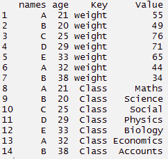
• gather() – it ‘gathers’ multiple columns. Then, it converts them into key:value pairs. This function will transform wide from of data to long form. You can use it as in alternative to ‘melt’ in reshape package.
• spread() – It does reverse of gather. It takes a key:value pair and converts it into separate columns.
• separate() – It splits a column into multiple columns.
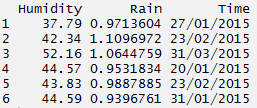
• unite() – It does reverse of separate. It unites multiple columns into single column

Let’s understand it closely using the code below:

#load package
> library(tidyr)

#create a dummy data set
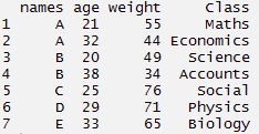
> names <- c('A','B','C','D','E','A','B')
> weight <- c(55,49,76,71,65,44,34)
> age <- c(21,20,25,29,33,32,38)
> Class <- c('Maths','Science','Social','Physics','Biology','Economics','Accounts')

#create data frame
> tdata <- data.frame(names, age, weight, Class)
> tdata



#using gather function
> long_t <- tdata %>% gather(Key, Value, weight:Class)
> long_t

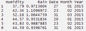
Separate function comes best in use when we are provided a date time variable in the data set. Since, the column contains multiple information, hence it makes sense to split it and use those values individually. Using the code below, I have separated a column into date, month and year.

#create a data set
> Humidity <- c(37.79, 42.34, 52.16, 44.57, 43.83, 44.59)
> Rain <- c(0.971360441, 1.10969716, 1.064475853, 0.953183435, 0.98878849, 0.939676146)
> Time <- c("27/01/2015 15:44","23/02/2015 23:24", "31/03/2015 19:15", "20/01/2015 20:52", "23/02/2015 07:46", "31/01/2015 01:55")

#build a data frame
> d_set <- data.frame(Humidity, Rain, Time)

#using separate function we can separate date, month, year
> separate_d <- d_set %>% separate(Time, c('Date', 'Month','Year'))
> separate_d



#using unite function - reverse of separate
> unite_d <- separate_d%>% unite(Time, c(Date, Month, Year), sep = "/")
> unite_d



#using spread function - reverse of gather
> wide_t <- long_t %>% spread(Key, Value)
> wide_t

Lubridate Package

Lubridate package reduces the pain of working of data time variable in R. The inbuilt function of this package offers a nice way to make easy parsing in dates and times. This packages is frequently used with data comprising of timely data. Here I have covered three basic tasks accomplished using Lubridate.

This includes update function, duration function and date extraction. As a beginner, knowing these 3 functions would give you good enough expertise to deal with time variables. Though, R has inbuilt functions for handling dates, but this is much faster. Let’s understand it using the code below:

> install.packages('lubridate')
> library(lubridate)

#current date and time
> now()
[1] "2015-12-11 13:23:48 IST"

#assigning current date and time to variable n_time
> n_time <- now()

#using update function
> n_update <- update(n_time, year = 2013, month = 10)
> n_update
[1] "2013-10-11 13:24:28 IST"

#add days, months, year, seconds
> d_time <- now()
> d_time + ddays(1)
[1] "2015-12-12 13:24:54 IST"
> d_time + dweeks(2)
[1] "2015-12-12 13:24:54 IST"

> d_time + dyears(3)
[1] "2018-12-10 13:24:54 IST"

> d_time + dhours(2)
[1] "2015-12-11 15:24:54 IST"

> d_time + dminutes(50)
[1] "2015-12-11 14:14:54 IST"

> d_time + dseconds(60)
[1] "2015-12-11 13:25:54 IST"

#extract date,time

> n_time$hour <- hour(now())
> n_time$minute <- minute(now())
> n_time$second <- second(now())
> n_time$month <- month(now())
> n_time$year <- year(now())

#check the extracted dates in separate columns
> new_data <- data.frame(n_time$hour, n_time$minute, n_time$second, n_time$month, n_time$year)
> new_data

Note: The best use of these packages is not in isolation but in conjunction. You could easily use this package with dplyr where you can easily select a data variable and extract the useful data from it using the chain command.

End Notes

These packages would not only enhance your data manipulation experience, but also give you reasons to explore R in depth. Now we have seen, these packages make coding in R easier. You no longer need to write long codes. Instead write short codes and do more.

Every package has multi tasking abilities. Hence, I would suggest you to get hold of important function which can be used frequently. And, once you get familiar with them, you can dig deeper. I did this mistake initially. I tried at exploring all the features in ggplot2 and ended up in a confusion. I’d suggest you to practice these codes as you read. This would help you build confidence on using these packages.

In this article, I’ve explained the use of 7 R packages which can make data exploration easier and faster. R known for its awesome statistical functions, with newly updated packages makes a favorite tool of data scientists too.

If you like what you just read & want to continue your analytics learning, subscribe to our emails, follow us on twitter or like our facebook page.