Step by step guide to building sentiment analysis model using graphlab

I have been using graph lab for quite some time now. The first Kaggle competition I used it for was Click Trough Rate (CTR) and I was amazed to see the speed at which it can crunch such big data. Over last few months, I have realised much broader applications of GraphLab. In this article I will take up the text mining capability of GraphLab and solve one of the Kaggle problems. I will be referring to this problem with a small tweak. The problem will classify the sentiment of each phrase into one of the 5 buckets. For simplicity, I will convert the sentiment into two category variable (with or without sentiment more than 3). This way I will be able to use all the classification algorithm of GraphLab in this exercise.

If you are completely new to GraphLab, I will recommend you to read this article before doing this exercise. Let’s look at the problem statement first.

Problem Statment

This problem is a very advanced problem of sentiment analysis, because it focuses to capture not so obvious trends. For instance sarcasm or frustration etc. And we do it by breaking down the sentence. For instance, if I say “The movie was OK but not that awesome” . What do you think is the sentiment of this sentence. It looks neutral as it was expected to be awesome but it was just fine. Now try this “The movie was OK”. Now the meaning of the sentence is quite different as now we don’t know what was author expecting of the movie. This problem gives many sentences broken down to phrases and sentiments of these phrases. This dataset just enables you to create your own sentiment miner algorithm. Here is how the problem reads on Kaggle –

"There's a thin line between likably old-fashioned and fuddy-duddy, and The Count of Monte Cristo ... never quite settles on either side."

The Rotten Tomatoes movie review dataset is a corpus of movie reviews used for sentiment analysis, originally collected by Pang and Lee [1]. In their work on sentiment treebanks, Socher et al. [2] used Amazon's Mechanical Turk to create fine-grained labels for all parsed phrases in the corpus. This competition presents a chance to benchmark your sentiment-analysis ideas on the Rotten Tomatoes dataset. You are asked to label phrases on a scale of five values: negative, somewhat negative, neutral, somewhat positive, positive. Obstacles like sentence negation, sarcasm, terseness, language ambiguity, and many others make this task very challenging.

Let’s get started

Let’s load the data and GraphLab.

The entire data set loads in less than 1 minute, which is amazing compared to 7 minutes on my R setup.

Now it’s time to convert sentiment into a two class flag variable.

convert = lambda x:1 if x>3 else 0

sf_train['target'] = sf_train['Sentiment'].apply(convert)
sf_train[111:190]

Now we start with the text mining on these phrases.

sf_train['word_count'] = graphlab.text_analytics.count_words(sf_train['Phrase'])

train,test = sf_train.random_split(0.6,seed=0)

len(train)

93517

basic_model = graphlab.logistic_classifier.create(train,target='target',features = ['word_count'])

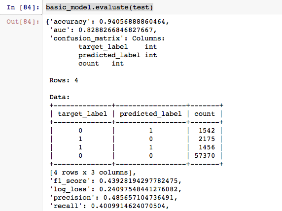
Now that we have our first model ready, let’s evaluate our model on various metrics.

Now, we will try a few more advanced techniques.

random_forest_1 = graphlab.random_forest_classifier.create(train, target='target',features = ['word_count'])

gbm_1 = graphlab.boosted_trees_classifier.create(train, target='target',features = ['word_count'])

svm_1 = graphlab.svm_classifier.create(train, target='target',features = ['word_count'])

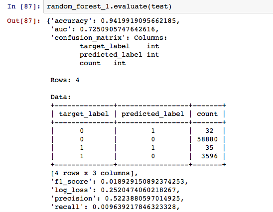
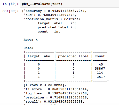
And we evaluate each of these models in the same way we did for logistic.

As you can observe from all the evaluations, with accuracy as the primary metric, GBM comes out to be the best model on the test data.

End Notes

My journey with GraphLab has been amazing till date. I will be soon publishing another article with Photo classification using GraphLab which I am currently working on.

Did you like this article? Have you used GraphLab before? If yes, how was the experience. Share with us applications you have used the tool GraphLab for.

If you like what you just read & want to continue your analytics learning, subscribe to our emails, follow us on twitter or like our facebook page.

Tavish Srivastava

Tavish Srivastava, co-founder and Chief Strategy Officer of Analytics Vidhya, is an IIT Madras graduate and a passionate data-science professional with 8+ years of diverse experience in markets including the US, India and Singapore, domains including Digital Acquisitions, Customer Servicing and Customer Management, and industry including Retail Banking, Credit Cards and Insurance. He is fascinated by the idea of artificial intelligence inspired by human intelligence and enjoys every discussion, theory or even movie related to this idea.