A Comprehensive Beginner’s Guide to Creating a Time Series Forecast (With Codes in Python and R)

27 minutes

Introduction

Time Series (referred as TS from now) is considered to be one of the less known skills in the data science space (Even I had little clue about it a couple of days back). I set myself on a journey to learn the basic steps for solving a Time Series problem and here I am sharing the same with you. These will definitely help you get a decent model in any future project you take up!

Before going through this article, I highly recommend reading A Complete Tutorial on Time Series Modeling in R and taking the free Time Series Forecasting course. It focuses on fundamental concepts and I will focus on using these concepts in solving a problem end-to-end along with codes in Python. Many resources exist for time series in R but very few are there for Python so I’ll be using Python in this article.

Are you a beginner looking for a place to start your data science journey? Here is a comprehensive course to assist you in your journey. Master Time Series, Machine Learning and Deep Learning through our Certified Blackbelt Program-

• Certified AI & ML Blackbelt+ Program

Learning Objectives:

• Learn the steps to create a Time Series forecast.
• Additional focus on Dickey-Fuller test & ARIMA (Autoregressive, moving average) models.
• Learn the concepts theoretically as well as with their implementation in python.

What Is Time Series?

As the name suggests, TS is a collection of data points collected at constant time intervals. These are analyzed to determine the long term trend so as to forecast the future or perform some other form of analysis. But what makes a TS different from say a regular regression problem? There are 2 things:

1. It is time dependent. So the basic assumption of a linear regression model that the observations are independent doesn’t hold in this case.
2. Along with an increasing or decreasing trend, most TS have some form of seasonality trends, i.e. variations specific to a particular time frame. For example, if you see the sales of a woolen jacket over time, you will invariably find higher sales in winter seasons.

Because of the inherent properties of a TS, there are various steps involved in analyzing it. These are discussed in detail below. Lets start by loading a TS object in Python. We’ll be using the popular AirPassengers data set which can be downloaded here.

Please note that the aim of this article is to familiarize you with the various techniques used for TS in general. The example considered here is just for illustration and I will focus on coverage a breadth of topics and not making a very accurate forecast.

Loading and Handling Time Series in Pandas

Pandas has dedicated libraries for handling TS objects, particularly the datatime64[ns] class which stores time information and allows us to perform some operations really fast. Lets start by firing up the required libraries:

Let’s understand the arguments one by one:

1. parse_dates: This specifies the column which contains the date-time information. As we say above, the column name is ‘Month’.
2. index_col: A key idea behind using Pandas for TS data is that the index has to be the variable depicting date-time information. So this argument tells pandas to use the ‘Month’ column as index.
3. date_parser: This specifies a function which converts an input string into datetime variable. Be default Pandas reads data in format ‘YYYY-MM-DD HH:MM:SS’. If the data is not in this format, the format has to be manually defined. Something similar to the dataparse function defined here can be used for this purpose.

Now we can see that the data has time object as index and #Passengers as the column. We can cross-check the datatype of the index with the following command:

data.index

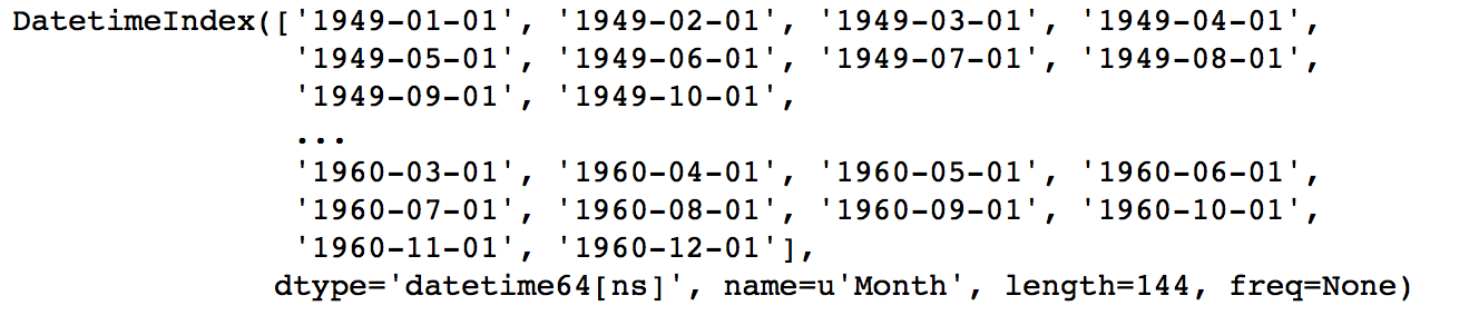
Notice the dtype=’datetime[ns]’ which confirms that it is a datetime object. As a personal preference, I would convert the column into a Series object to prevent referring to columns names every time I use the TS. Please feel free to use as a dataframe is that works better for you.

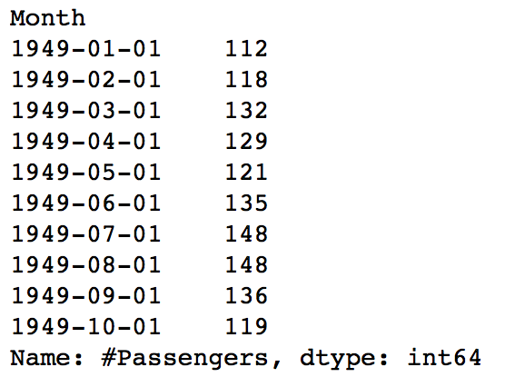
ts = data[‘#Passengers’]
ts.head(10)

Before going further, I’ll discuss some indexing techniques for TS data. Lets start by selecting a particular value in the Series object. This can be done in following 2 ways:

#1. Specific the index as a string constant:
ts['1949-01-01']

#2. Import the datetime library and use 'datetime' function:
from datetime import datetime
ts[datetime(1949,1,1)]

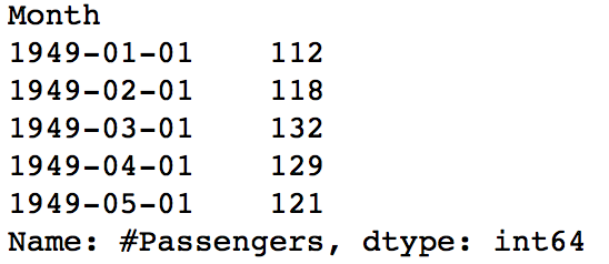
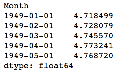
Both would return the value ‘112’ which can also be confirmed from previous output. Suppose we want all the data upto May 1949. This can be done in 2 ways:

#1. Specify the entire range:
ts['1949-01-01':'1949-05-01']

#2. Use ':' if one of the indices is at ends:
ts[:'1949-05-01']

Both would yield following output:

There are 2 things to note here:

1. Unlike numeric indexing, the end index is included here. For instance, if we index a list as a[:5] then it would return the values at indices – [0,1,2,3,4]. But here the index ‘1949-05-01’ was included in the output.
2. The indices have to be sorted for ranges to work. If you randomly shuffle the index, this won’t work.

Consider another instance where you need all the values of the year 1949. This can be done as:

ts['1949']

The month part was omitted. Similarly if you all days of a particular month, the day part can be omitted.

Now, lets move onto the analyzing the TS.

How to Check the Stationarity of a Time Series?

A TS is said to be stationary if its statistical properties such as mean, variance remain constant over time. But why is it important? Most of the TS models work on the assumption that the TS is stationary. Intuitively, we can sat that if a TS has a particular behaviour over time, there is a very high probability that it will follow the same in the future. Also, the theories related to stationary series are more mature and easier to implement as compared to non-stationary series.

Stationarity is defined using very strict criterion. However, for practical purposes we can assume the series to be stationary if it has constant statistical properties over time, ie. the following:

1. constant mean
2. constant variance
3. an autocovariance that does not depend on time.

I’ll skip the details as it is very clearly defined in this article. Lets move onto the ways of testing stationarity. First and foremost is to simple plot the data and analyze visually. The data can be plotted using following command:

plt.plot(ts)

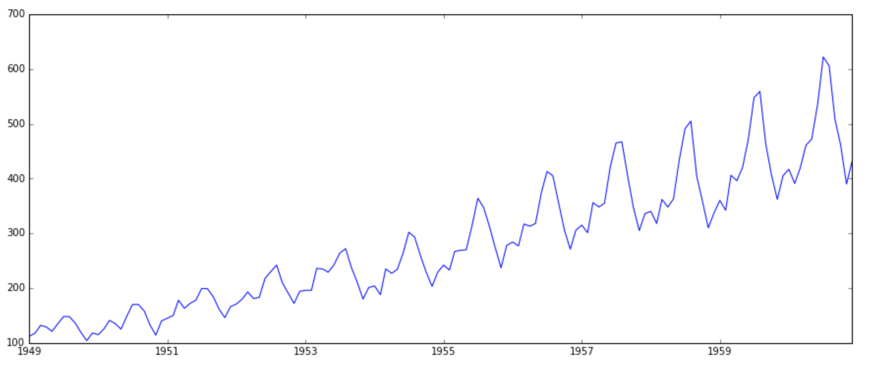
It is clearly evident that there is an overall increasing trend in the data along with some seasonal variations. However, it might not always be possible to make such visual inferences (we’ll see such cases later). So, more formally, we can check stationarity using the following:

1. Plotting Rolling Statistics: We can plot the moving average or moving variance and see if it varies with time. By moving average/variance I mean that at any instant ‘t’, we’ll take the average/variance of the last year, i.e. last 12 months. But again this is more of a visual technique.
2. Dickey-Fuller Test: This is one of the statistical tests for checking stationarity. Here the null hypothesis is that the TS is non-stationary. The test results comprise of a Test Statistic and some Critical Values for difference confidence levels. If the ‘Test Statistic’ is less than the ‘Critical Value’, we can reject the null hypothesis and say that the series is stationary. Refer this article for details.

These concepts might not sound very intuitive at this point. I recommend going through the prequel article. If you’re interested in some theoretical statistics, you can refer Introduction to Time Series and Forecasting by Brockwell and Davis. The book is a bit stats-heavy, but if you have the skill to read-between-lines, you can understand the concepts and tangentially touch the statistics.

Back to checking stationarity, we’ll be using the rolling statistics plots along with Dickey-Fuller test results a lot so I have defined a function which takes a TS as input and generated them for us. Please note that I’ve plotted standard deviation instead of variance to keep the unit similar to mean.

from statsmodels.tsa.stattools import adfuller
def test_stationarity(timeseries):
    
    #Determing rolling statistics
    rolmean = pd.rolling_mean(timeseries, window=12)
    rolstd = pd.rolling_std(timeseries, window=12)

    #Plot rolling statistics:
    orig = plt.plot(timeseries, color='blue',label='Original')
    mean = plt.plot(rolmean, color='red', label='Rolling Mean')
    std = plt.plot(rolstd, color='black', label = 'Rolling Std')
    plt.legend(loc='best')
    plt.title('Rolling Mean & Standard Deviation')
    plt.show(block=False)
    
    #Perform Dickey-Fuller test:
    print 'Results of Dickey-Fuller Test:'
    dftest = adfuller(timeseries, autolag='AIC')
    dfoutput = pd.Series(dftest[0:4], index=['Test Statistic','p-value','#Lags Used','Number of Observations Used'])
    for key,value in dftest[4].items():
        dfoutput['Critical Value (%s)'%key] = value
    print dfoutput

The code is pretty straight forward. Please feel free to discuss the code in comments if you face challenges in grasping it.

Let’s run it for our input series:

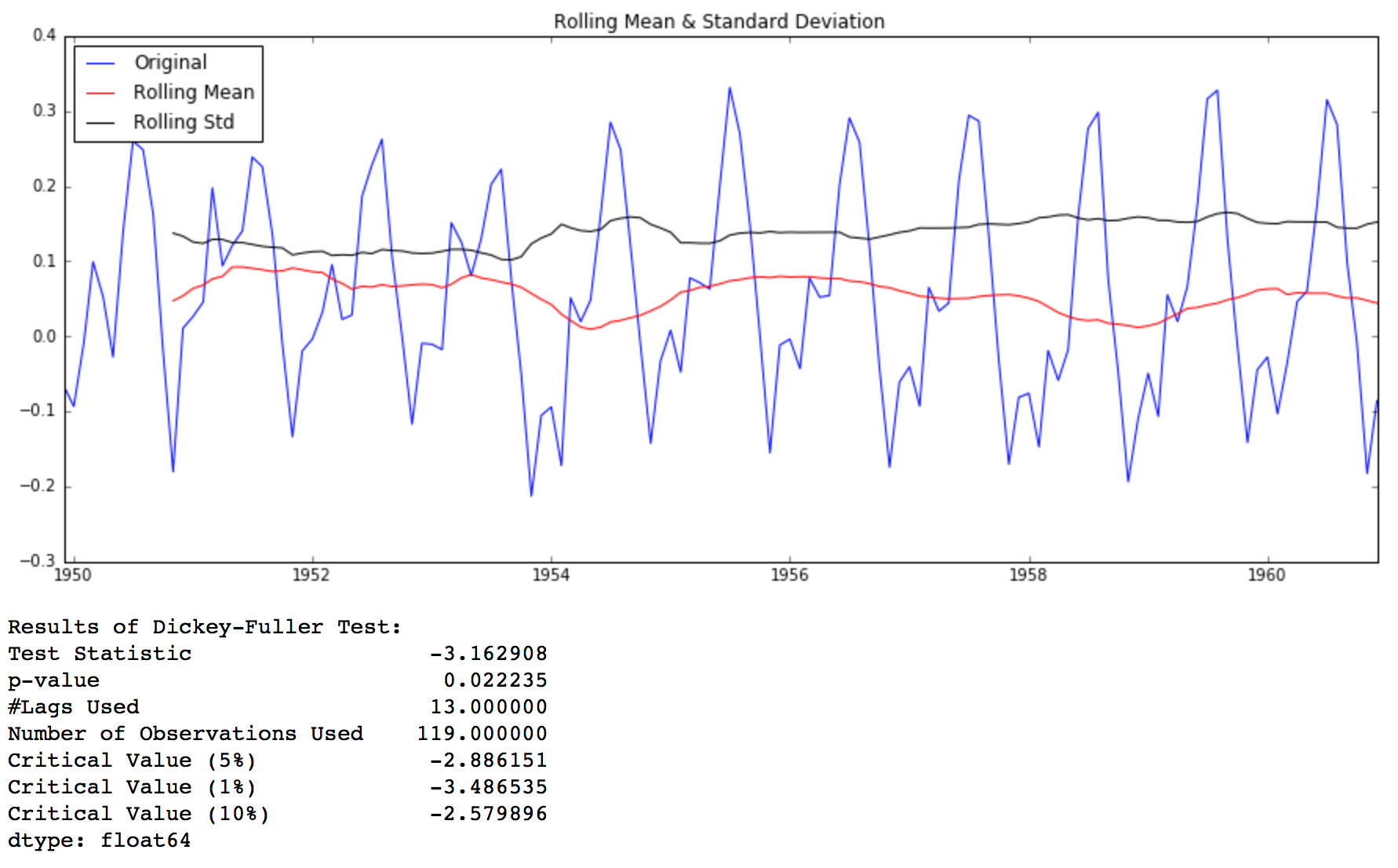
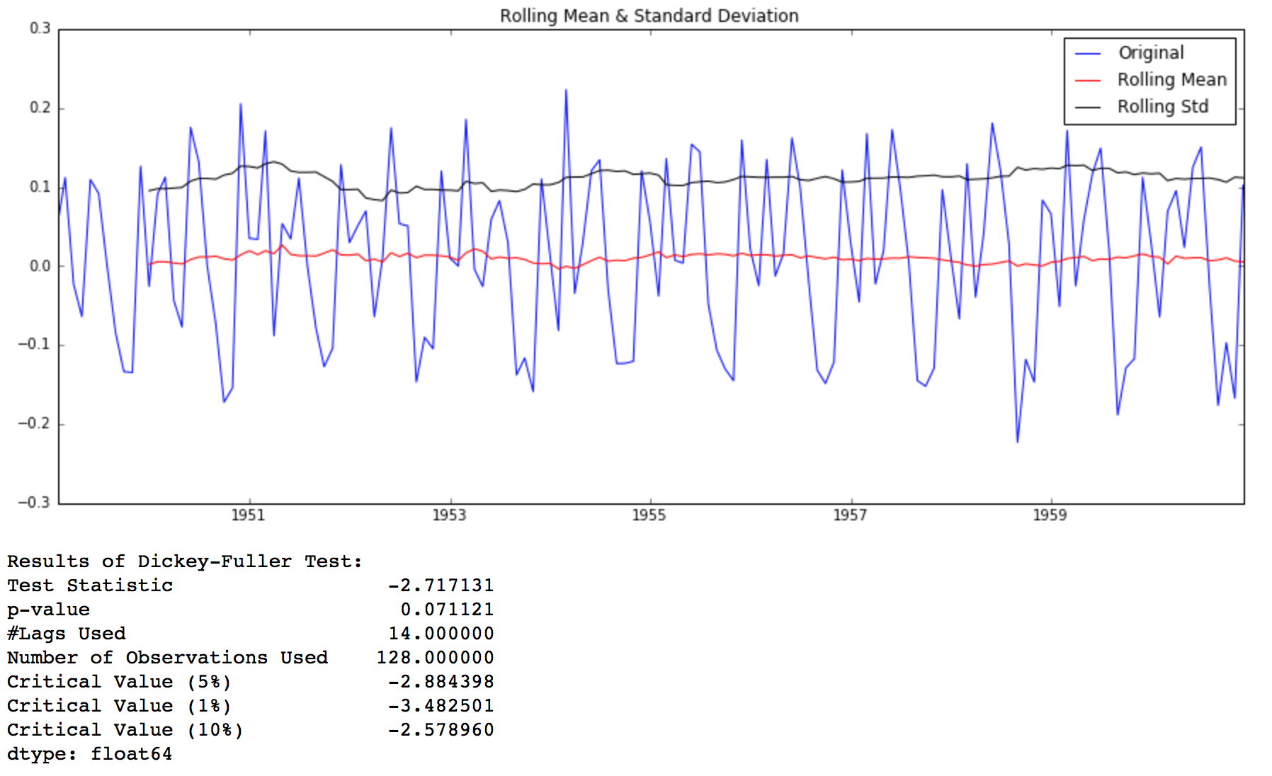
test_stationarity(ts)

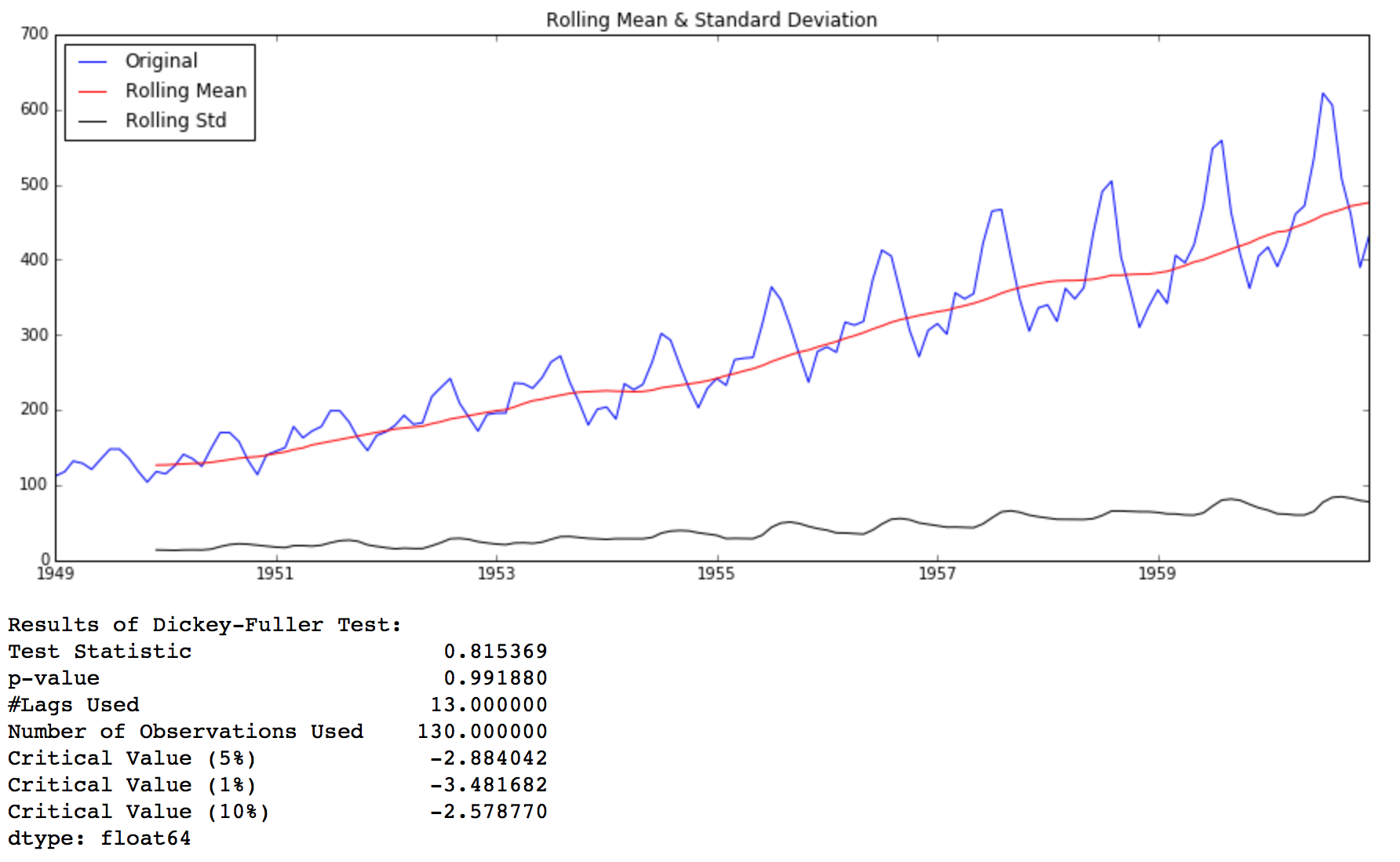
Though the variation in standard deviation is small, mean is clearly increasing with time and this is not a stationary series. Also, the test statistic is way more than the critical values. Note that the signed values should be compared and not the absolute values.

Next, we’ll discuss the techniques that can be used to take this TS towards stationarity.

How to Make a Time Series Stationary?

Though stationarity assumption is taken in many TS models, almost none of practical time series are stationary. So statisticians have figured out ways to make series stationary, which we’ll discuss now. Actually, its almost impossible to make a series perfectly stationary, but we try to take it as close as possible.

Lets understand what is making a TS non-stationary. There are 2 major reasons behind non-stationaruty of a TS:
1. Trend – varying mean over time. For eg, in this case we saw that on average, the number of passengers was growing over time.
2. Seasonality – variations at specific time-frames. eg people might have a tendency to buy cars in a particular month because of pay increment or festivals.

The underlying principle is to model or estimate the trend and seasonality in the series and remove those from the series to get a stationary series. Then statistical forecasting techniques can be implemented on this series. The final step would be to convert the forecasted values into the original scale by applying trend and seasonality constraints back.

Note: I’ll be discussing a number of methods. Some might work well in this case and others might not. But the idea is to get a hang of all the methods and not focus on just the problem at hand.

Let’s start by working on the trend part.

Estimating & Eliminating Trend

One of the first tricks to reduce trend can be transformation. For example, in this case we can clearly see that the there is a significant positive trend. So we can apply transformation which penalize higher values more than smaller values. These can be taking a log, square root, cube root, etc. Lets take a log transform here for simplicity:

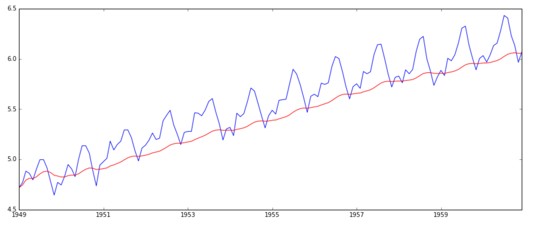
ts_log = np.log(ts)
plt.plot(ts_log)

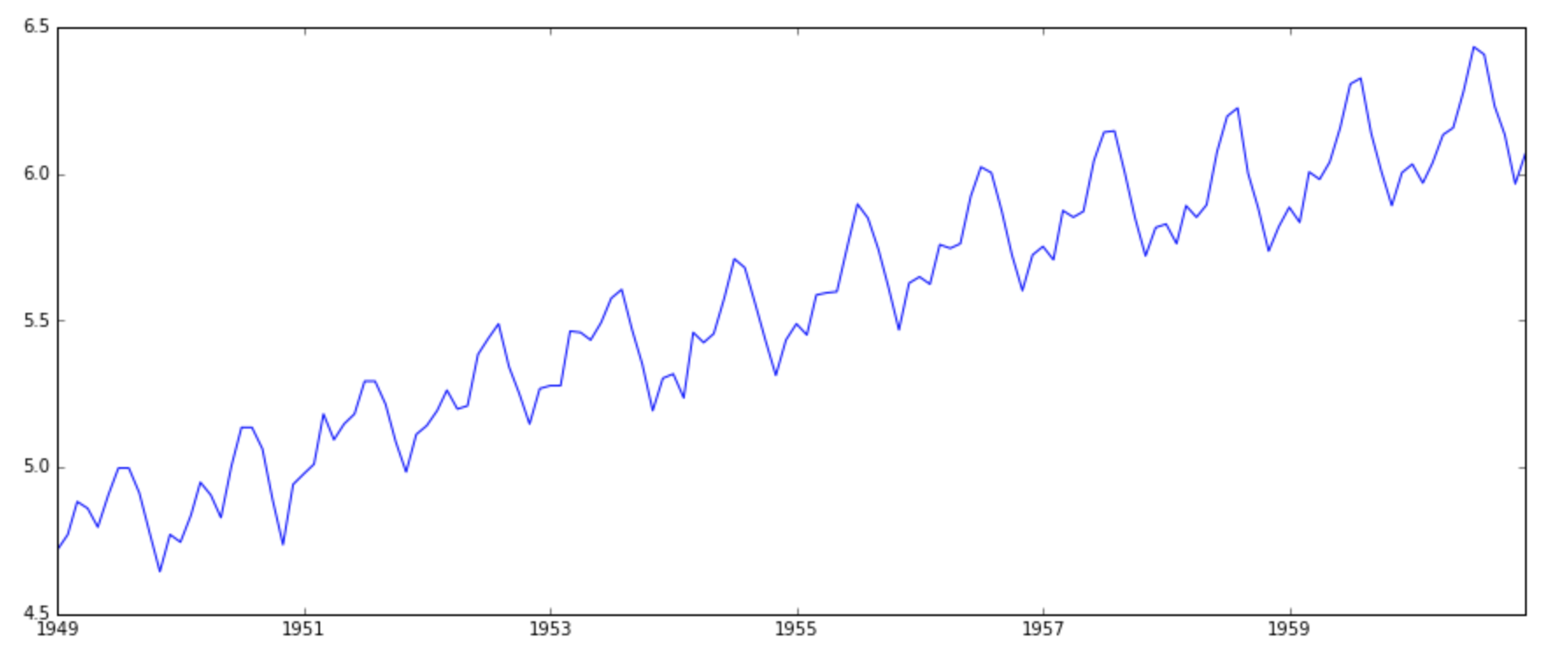
In this simpler case, it is easy to see a forward trend in the data. But its not very intuitive in presence of noise. So we can use some techniques to estimate or model this trend and then remove it from the series. There can be many ways of doing it and some of most commonly used are:

1. Aggregation – taking average for a time period like monthly/weekly averages
2. Smoothing – taking rolling averages
3. Polynomial Fitting – fit a regression model

I will discuss smoothing here and you should try other techniques as well which might work out for other problems. Smoothing refers to taking rolling estimates, i.e. considering the past few instances. There are can be various ways but I will discuss two of those here.

Moving Average

In this approach, we take average of ‘k’ consecutive values depending on the frequency of time series. Here we can take the average over the past 1 year, i.e. last 12 values. Pandas has specific functions defined for determining rolling statistics.

moving_avg = pd.rolling_mean(ts_log,12)
plt.plot(ts_log)
plt.plot(moving_avg, color='red')

The red line shows the rolling mean. Lets subtract this from the original series. Note that since we are taking average of last 12 values, rolling mean is not defined for first 11 values. This can be observed as:

ts_log_moving_avg_diff = ts_log - moving_avg
ts_log_moving_avg_diff.head(12)

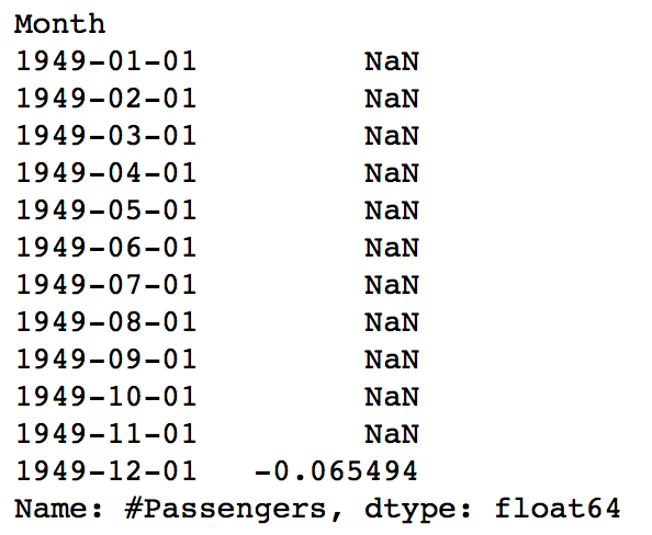
Notice the first 11 being Nan. Lets drop these NaN values and check the plots to test stationarity.

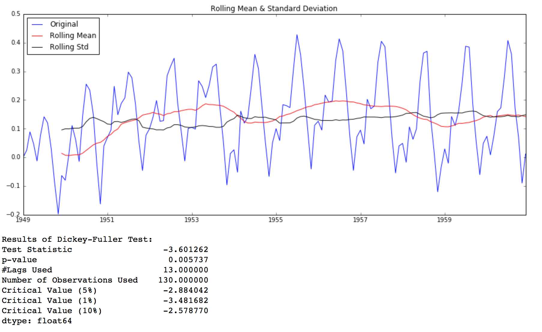
ts_log_moving_avg_diff.dropna(inplace=True)
test_stationarity(ts_log_moving_avg_diff)

This looks like a much better series. The rolling values appear to be varying slightly but there is no specific trend. Also, the test statistic is smaller than the 5% critical values so we can say with 95% confidence that this is a stationary series.

However, a drawback in this particular approach is that the time-period has to be strictly defined. In this case we can take yearly averages but in complex situations like forecasting a stock price, its difficult to come up with a number. So we take a ‘weighted moving average’ where more recent values are given a higher weight. There can be many technique for assigning weights. A popular one is exponentially weighted moving average where weights are assigned to all the previous values with a decay factor. Find details here. This can be implemented in Pandas as:

expwighted_avg = pd.ewma(ts_log, halflife=12)
plt.plot(ts_log)
plt.plot(expwighted_avg, color='red')

Note that here the parameter ‘halflife’ is used to define the amount of exponential decay. This is just an assumption here and would depend largely on the business domain. Other parameters like span and center of mass can also be used to define decay which are discussed in the link shared above. Now, let’s remove this from series and check stationarity:

ts_log_ewma_diff = ts_log - expwighted_avg
test_stationarity(ts_log_ewma_diff)

This TS has even lesser variations in mean and standard deviation in magnitude. Also, the test statistic is smaller than the 1% critical value, which is better than the previous case. Note that in this case, there will be no missing values as all values from starting are given weights. So it’ll work even with no previous values.

Eliminating Trend and Seasonality

The simple trend reduction techniques discussed before don’t work in all cases, particularly the ones with high seasonality. Let’s discuss two ways of removing trend and seasonality:

1. Differencing – taking the difference with a particular time lag
2. Decomposition – modeling both trend and seasonality and removing them from the model

Differencing

One of the most common methods of dealing with both trend and seasonality is differencing. In this technique, we take the difference of the observation at a particular instant with that at the previous instant. This mostly works well in improving stationarity. First-order differencing can be done in Pandas as:

ts_log_diff = ts_log - ts_log.shift()
plt.plot(ts_log_diff)

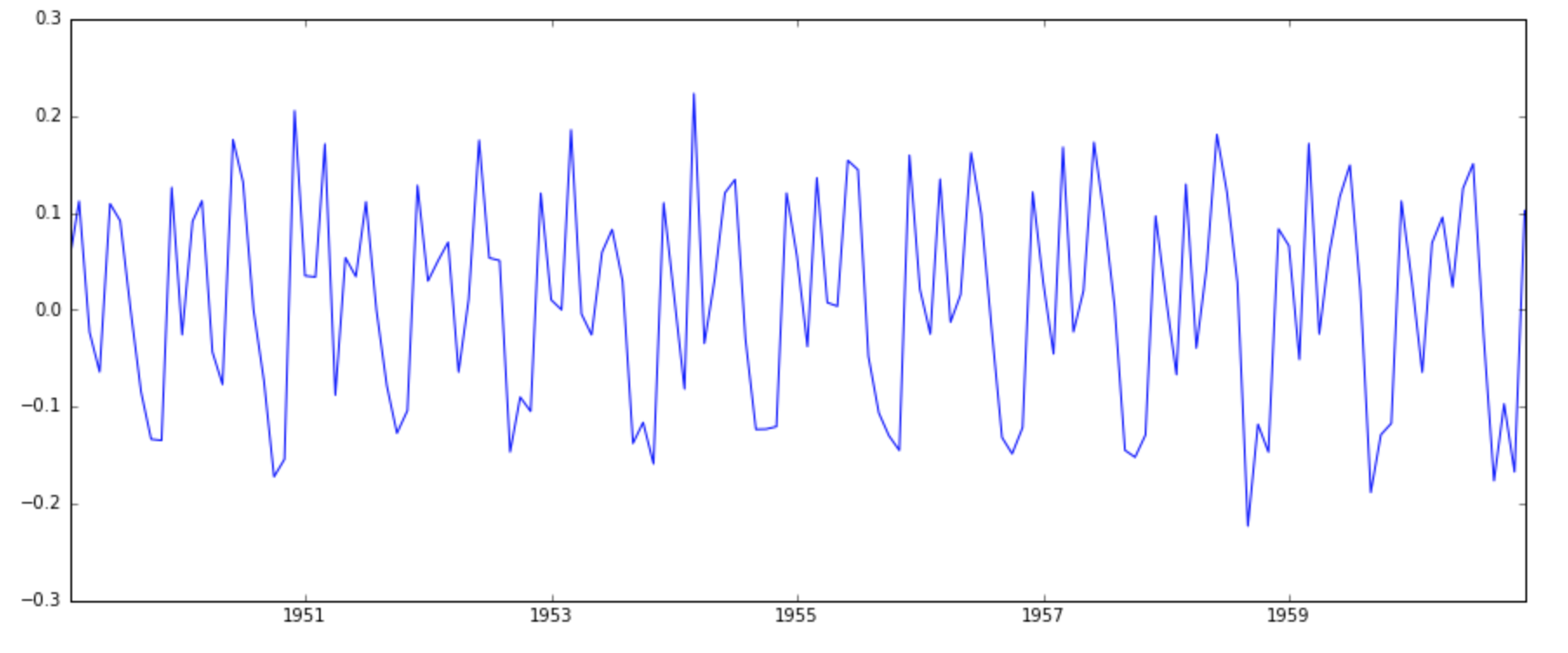
This appears to have reduced trend considerably. Lets verify using our plots:

ts_log_diff.dropna(inplace=True)
test_stationarity(ts_log_diff)

We can see that the mean and std variations have small variations with time. Also, the Dickey-Fuller test statistic is less than the 10% critical value, thus the TS is stationary with 90% confidence. We can also take second or third order differences which might get even better results in certain applications. I leave it to you to try them out.

Decomposing

In this approach, both trend and seasonality are modeled separately and the remaining part of the series is returned. I’ll skip the statistics and come to the results:

from statsmodels.tsa.seasonal import seasonal_decompose
decomposition = seasonal_decompose(ts_log)

trend = decomposition.trend
seasonal = decomposition.seasonal
residual = decomposition.resid

plt.subplot(411)
plt.plot(ts_log, label='Original')
plt.legend(loc='best')
plt.subplot(412)
plt.plot(trend, label='Trend')
plt.legend(loc='best')
plt.subplot(413)
plt.plot(seasonal,label='Seasonality')
plt.legend(loc='best')
plt.subplot(414)
plt.plot(residual, label='Residuals')
plt.legend(loc='best')
plt.tight_layout()

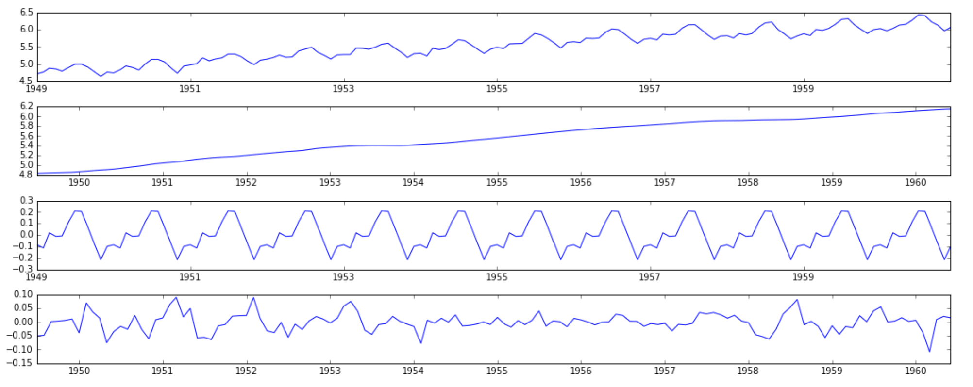
Here we can see that the trend, seasonality are separated out from data and we can model the residuals. Lets check stationarity of residuals:

ts_log_decompose = residual
ts_log_decompose.dropna(inplace=True)
test_stationarity(ts_log_decompose)

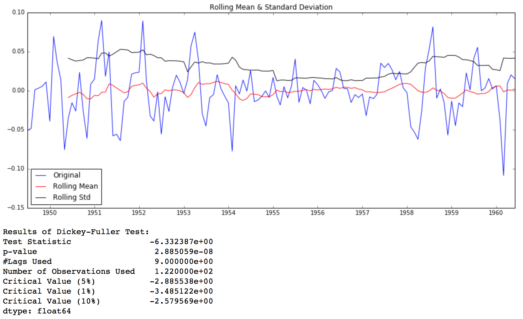
The Dickey-Fuller test statistic is significantly lower than the 1% critical value. So this TS is very close to stationary. You can try advanced decomposition techniques as well which can generate better results. Also, you should note that converting the residuals into original values for future data in not very intuitive in this case.

Forecasting a Time Series

We saw different techniques and all of them worked reasonably well for making the TS stationary. Lets make model on the TS after differencing as it is a very popular technique. Also, its relatively easier to add noise and seasonality back into predicted residuals in this case. Having performed the trend and seasonality estimation techniques, there can be two situations:

1. A strictly stationary series with no dependence among the values. This is the easy case wherein we can model the residuals as white noise. But this is very rare.
2. A series with significant dependence among values. In this case we need to use some statistical models like ARIMA to forecast the data.

Let me give you a brief introduction to ARIMA. I won’t go into the technical details but you should understand these concepts in detail if you wish to apply them more effectively. ARIMA stands for Auto-Regressive Integrated Moving Averages. The ARIMA forecasting for a stationary time series is nothing but a linear (like a linear regression) equation. The predictors depend on the parameters (p,d,q) of the ARIMA model:

1. Number of AR (Auto-Regressive) terms (p): AR terms are just lags of dependent variable. For instance if p is 5, the predictors for x(t) will be x(t-1)….x(t-5).
2. Number of MA (Moving Average) terms (q): MA terms are lagged forecast errors in prediction equation. For instance if q is 5, the predictors for x(t) will be e(t-1)….e(t-5) where e(i) is the difference between the moving average at i^th instant and actual value.
3. Number of Differences (d): These are the number of nonseasonal differences, i.e. in this case we took the first order difference. So either we can pass that variable and put d=0 or pass the original variable and put d=1. Both will generate same results.

An importance concern here is how to determine the value of ‘p’ and ‘q’. We use two plots to determine these numbers. Lets discuss them first.

1. Autocorrelation Function (ACF): It is a measure of the correlation between the the TS with a lagged version of itself. For instance at lag 5, ACF would compare series at time instant ‘t1’…’t2’ with series at instant ‘t1-5’…’t2-5’ (t1-5 and t2 being end points).
2. Partial Autocorrelation Function (PACF): This measures the correlation between the TS with a lagged version of itself but after eliminating the variations already explained by the intervening comparisons. Eg at lag 5, it will check the correlation but remove the effects already explained by lags 1 to 4.

The ACF and PACF plots for the TS after differencing can be plotted as:

#ACF and PACF plots:
from statsmodels.tsa.stattools import acf, pacf

lag_acf = acf(ts_log_diff, nlags=20)
lag_pacf = pacf(ts_log_diff, nlags=20, method='ols')

#Plot ACF: 
plt.subplot(121) 
plt.plot(lag_acf)
plt.axhline(y=0,linestyle='--',color='gray')
plt.axhline(y=-1.96/np.sqrt(len(ts_log_diff)),linestyle='--',color='gray')
plt.axhline(y=1.96/np.sqrt(len(ts_log_diff)),linestyle='--',color='gray')
plt.title('Autocorrelation Function')

#Plot PACF:
plt.subplot(122)
plt.plot(lag_pacf)
plt.axhline(y=0,linestyle='--',color='gray')
plt.axhline(y=-1.96/np.sqrt(len(ts_log_diff)),linestyle='--',color='gray')
plt.axhline(y=1.96/np.sqrt(len(ts_log_diff)),linestyle='--',color='gray')
plt.title('Partial Autocorrelation Function')
plt.tight_layout()

In this plot, the two dotted lines on either sides of 0 are the confidence interevals. These can be used to determine the ‘p’ and ‘q’ values as:

1. p – The lag value where the PACF chart crosses the upper confidence interval for the first time. If you notice closely, in this case p=2.
2. q – The lag value where the ACF chart crosses the upper confidence interval for the first time. If you notice closely, in this case q=2.

Now, lets make 3 different ARIMA models considering individual as well as combined effects. I will also print the RSS for each. Please note that here RSS is for the values of residuals and not actual series.

We need to load the ARIMA model first:

from statsmodels.tsa.arima_model import ARIMA

The p,d,q values can be specified using the order argument of ARIMA which take a tuple (p,d,q). Let model the 3 cases:

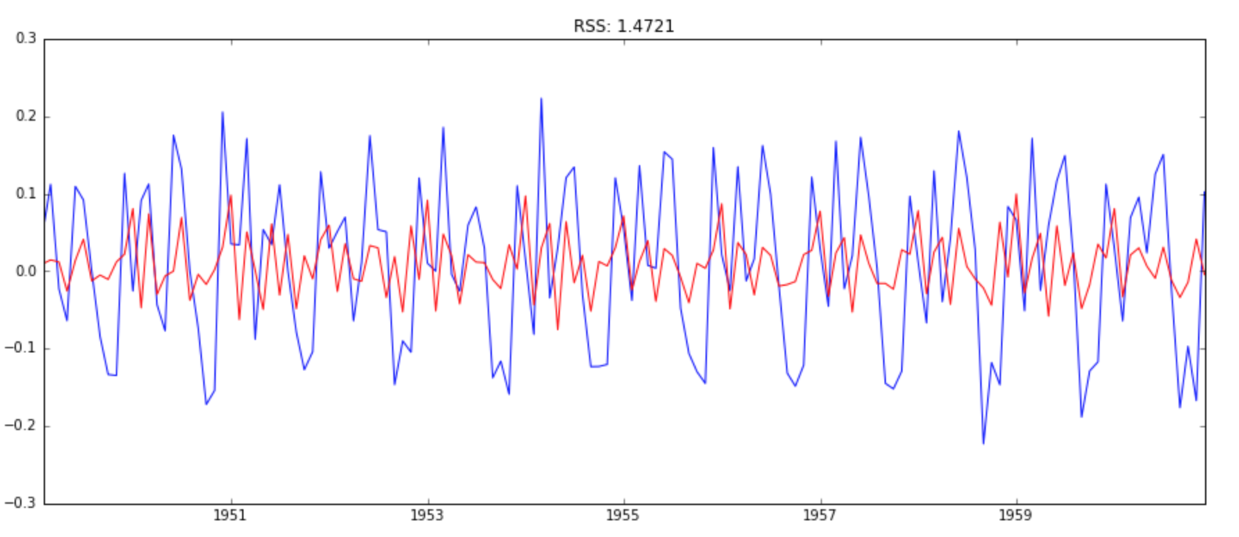
AR Model

model = ARIMA(ts_log, order=(2, 1, 0))  
results_AR = model.fit(disp=-1)  
plt.plot(ts_log_diff)
plt.plot(results_AR.fittedvalues, color='red')
plt.title('RSS: %.4f'% sum((results_AR.fittedvalues-ts_log_diff)**2))

MA Model

model = ARIMA(ts_log, order=(0, 1, 2))  
results_MA = model.fit(disp=-1)  
plt.plot(ts_log_diff)
plt.plot(results_MA.fittedvalues, color='red')
plt.title('RSS: %.4f'% sum((results_MA.fittedvalues-ts_log_diff)**2))

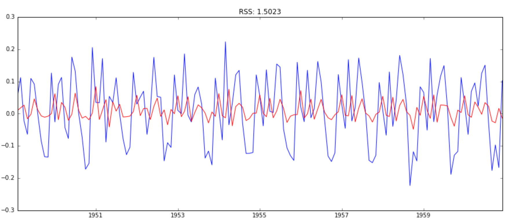
Combined Model

model = ARIMA(ts_log, order=(2, 1, 2))  
results_ARIMA = model.fit(disp=-1)  
plt.plot(ts_log_diff)
plt.plot(results_ARIMA.fittedvalues, color='red')
plt.title('RSS: %.4f'% sum((results_ARIMA.fittedvalues-ts_log_diff)**2))

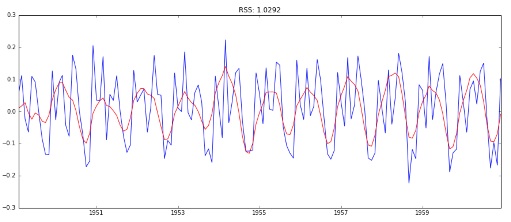
Here we can see that the AR and MA models have almost the same RSS but combined is significantly better. Now, we are left with 1 last step, i.e. taking these values back to the original scale.

Taking it back to original scale

Since the combined model gave best result, lets scale it back to the original values and see how well it performs there. First step would be to store the predicted results as a separate series and observe it.

predictions_ARIMA_diff = pd.Series(results_ARIMA.fittedvalues, copy=True)
print predictions_ARIMA_diff.head()

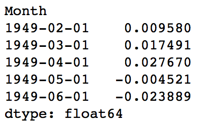
Notice that these start from ‘1949-02-01’ and not the first month. Why? This is because we took a lag by 1 and first element doesn’t have anything before it to subtract from. The way to convert the differencing to log scale is to add these differences consecutively to the base number. An easy way to do it is to first determine the cumulative sum at index and then add it to the base number. The cumulative sum can be found as:

predictions_ARIMA_diff_cumsum = predictions_ARIMA_diff.cumsum()
print predictions_ARIMA_diff_cumsum.head()

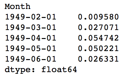
You can quickly do some back of mind calculations using previous output to check if these are correct. Next we’ve to add them to base number. For this lets create a series with all values as base number and add the differences to it. This can be done as:

predictions_ARIMA_log = pd.Series(ts_log.ix[0], index=ts_log.index)
predictions_ARIMA_log = predictions_ARIMA_log.add(predictions_ARIMA_diff_cumsum,fill_value=0)
predictions_ARIMA_log.head()

Here the first element is base number itself and from thereon the values cumulatively added. Last step is to take the exponent and compare with the original series.

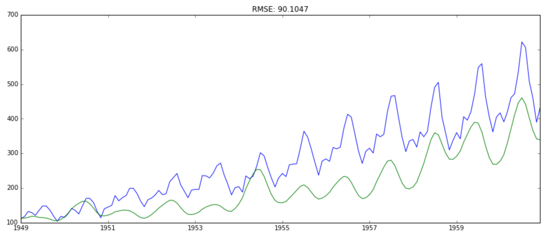
predictions_ARIMA = np.exp(predictions_ARIMA_log)
plt.plot(ts)
plt.plot(predictions_ARIMA)
plt.title('RMSE: %.4f'% np.sqrt(sum((predictions_ARIMA-ts)**2)/len(ts)))

That’s all in Python. Well, let’s learn how to implement a time series forecast in R.

Time Series Forecast in R

Step 1: Reading data and calculating basic summary

Output

class(tsdata)
"ts"
> #Observations of the time series data
> tsdata
Jan Feb Mar Apr May Jun Jul Aug Sep Oct Nov Dec
1949 112 118 132 129 121 135 148 148 136 119 104 118
1950 115 126 141 135 125 149 170 170 158 133 114 140
1951 145 150 178 163 172 178 199 199 184 162 146 166
1952 171 180 193 181 183 218 230 242 209 191 172 194
1953 196 196 236 235 229 243 264 272 237 211 180 201
1954 204 188 235 227 234 264 302 293 259 229 203 229
1955 242 233 267 269 270 315 364 347 312 274 237 278
1956 284 277 317 313 318 374 413 405 355 306 271 306
1957 315 301 356 348 355 422 465 467 404 347 305 336
1958 340 318 362 348 363 435 491 505 404 359 310 337
1959 360 342 406 396 420 472 548 559 463 407 362 405
1960 417 391 419 461 472 535 622 606 508 461 390 432
> #Summary of the data and missi

tsdata was converted to a data frame
Data Frame Summary 
tsdata 
Dimensions: 144 x 1 
Duplicates: 26

----------------------------------------------------------------------------------------------------
No Variable Stats / Values Freqs (% of Valid) Graph Valid Missing 
---- ---------- -------------------------- ----------------------- --------------------- -------- --
1 tsdata Mean (sd) : 280.3 (120) 118 distinct values . : . 144 0 
[ts] min < med < max: Start: 1949-01 : : . . : (100%) (0%) 
104 < 265.5 < 622 End : 1960-12 : : : : : 
IQR (CV) : 180.5 (0.4) : : : : : : : 
: : : : : : : : . . 
----------------------------------------------------------------------------------------------------

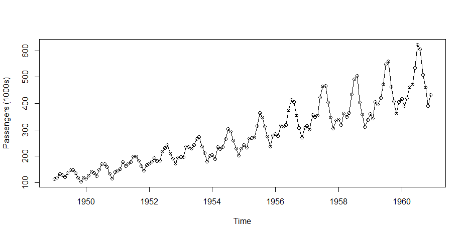
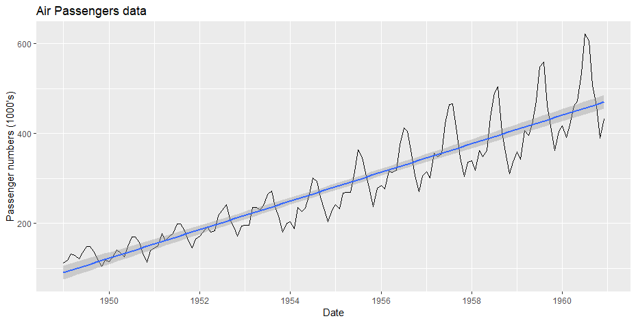
Step 2: Checking the cycle of Time Series Data and Plotting the Raw Data

Output

cycle(tsdata)
Jan Feb Mar Apr May Jun Jul Aug Sep Oct Nov Dec
1949 1 2 3 4 5 6 7 8 9 10 11 12
1950 1 2 3 4 5 6 7 8 9 10 11 12
1951 1 2 3 4 5 6 7 8 9 10 11 12
1952 1 2 3 4 5 6 7 8 9 10 11 12
1953 1 2 3 4 5 6 7 8 9 10 11 12
1954 1 2 3 4 5 6 7 8 9 10 11 12
1955 1 2 3 4 5 6 7 8 9 10 11 12
1956 1 2 3 4 5 6 7 8 9 10 11 12
1957 1 2 3 4 5 6 7 8 9 10 11 12
1958 1 2 3 4 5 6 7 8 9 10 11 12
1959 1 2 3 4 5 6 7 8 9 10 11 12
1960 1 2 3 4 5 6 7 8 9 10 11 12

Step 3: Decomposing the time series data

Output

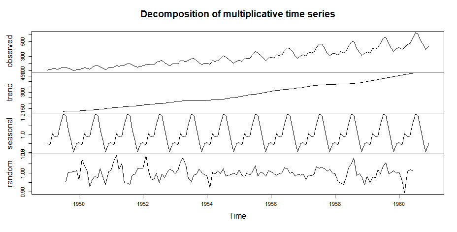
Step 4: Test the stationarity of data

Output

Augmented Dickey-Fuller Test

data: tsdata
Dickey-Fuller = -7.3186, Lag order = 5, p-value = 0.01
alternative hypothesis: stationary

the p-value is 0.01 which is <0.05, therefore, we reject the null hypothesis and hence time series is stationary.

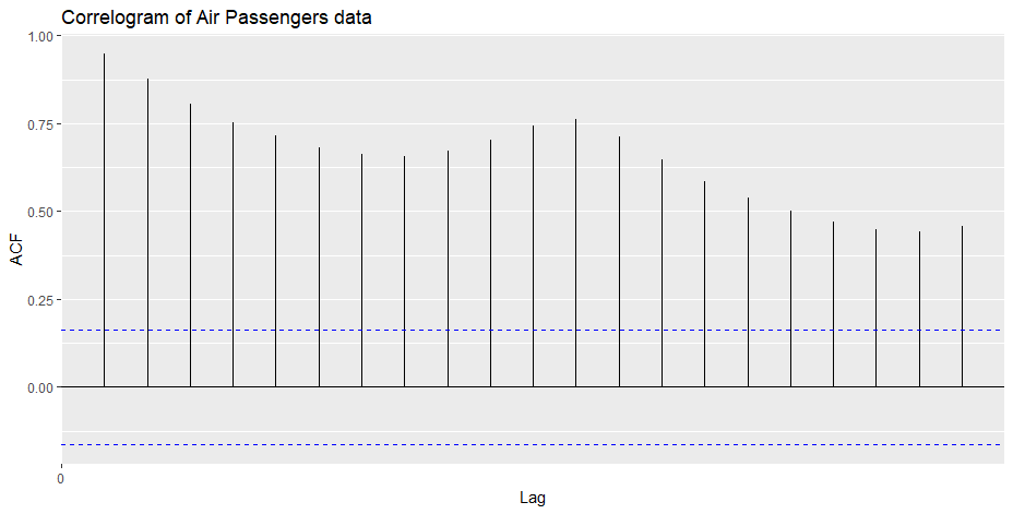
The maximum lag is at 1 or 12 months, indicates a positive relationship with the 12-month cycle.

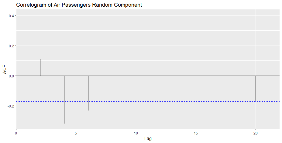
Autoplot the random time series observations from 7:138 which exclude the NA values

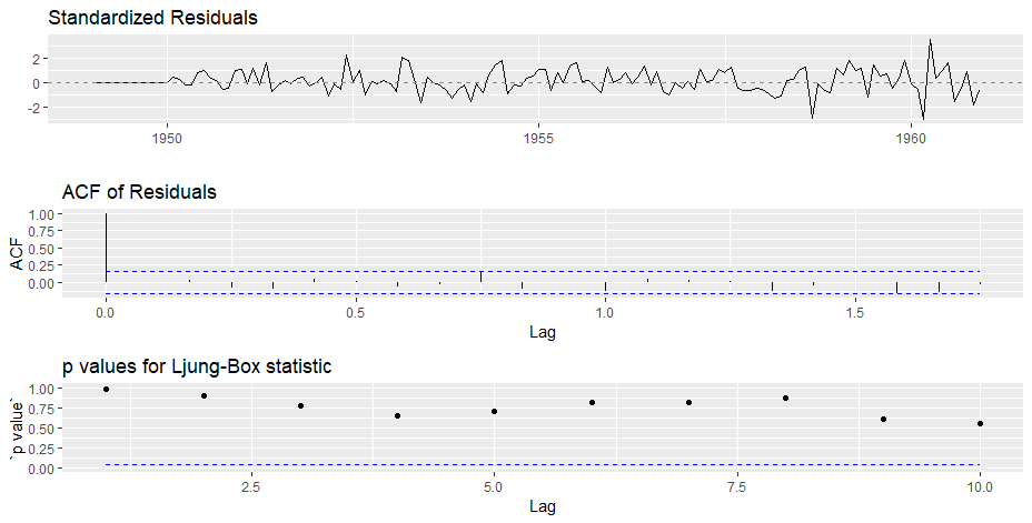
Step 5: Fitting the model

Output

Series: tsdata 
ARIMA(2,1,1)(0,1,0)[12]

Coefficients:
ar1 ar2 ma1
0.5960 0.2143 -0.9819
s.e. 0.0888 0.0880 0.0292

sigma^2 estimated as 132.3: log likelihood=-504.92
AIC=1017.85 AICc=1018.17 BIC=1029.35

Step 6: Forecasting

Output

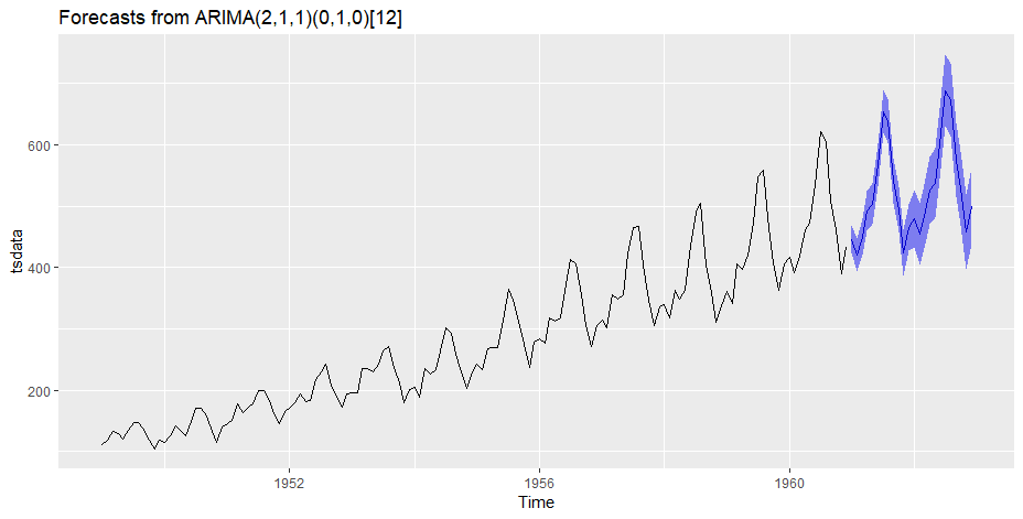
Finally we have a forecast at the original scale. Not a very good forecast I would say but you got the idea right? Now, I leave it upto you to refine the methodology further and make a better solution.

Sample Projects

Now, its time to take the plunge and actually play with some other real datasets. So are you ready to take on the challenge? Test the techniques discussed in this post and accelerate your learning in Time Series Analysis with the following Practice Problems:

	Practice Problem: Food Demand Forecasting Challenge	Forecast the demand of meals for a meal delivery company
	Practice Problem: Time Series Analyses	Forecast the passenger traffic for an intra-city rail system

Conclusion

Through this article I have tried to give you a standard approach for solving time series problem. This couldn’t have come at a better time as today is our Mini DataHack which will challenge you to solve a similar problem. We’ve covered concepts of stationarity, how to take a time series closer to stationarity and finally forecasting the residuals. It was a long journey and I skipped some statistical details which I encourage you to refer using the suggested material. If you don’t want to copy-paste, you can download the iPython notebook with all the codes from my GitHub repository.

Frequently Asked Questions

Aarshay 02 May, 2023