Introduction
Did you know the first neural network was discovered in early 1950s ?
Deep Learning (DL) and Neural Network (NN) is currently driving some of the most ingenious inventions in today’s century. Their incredible ability to learn from data and environment makes them the first choice of machine learning scientists.
Deep Learning and Neural Network lies in the heart of products such as self driving cars, image recognition software, recommender systems etc. Evidently, being a powerful algorithm, it is highly adaptive to various data types as well.
People think neural network is an extremely difficult topic to learn. Therefore, either some of them don’t use it, or the ones who use it, use it as a black box. Is there any point in doing something without knowing how is it done? NO!
In this article, I’ve attempted to explain the concept of neural network in simple words. Understanding this article requires a little bit of biology and lots of patience. By end of this article, you would become a confident analyst ready to start working with neural networks. In case you don’t understand anything, I’m always available in comments section.
Note: This article is best suited for intermediate users in data science & machine learning. Beginners might find it challenging.

Table of contents
What is a Neural Network?
Neural Networks (NN), also called as Artificial Neural Network is named after its artificial representation of working of a human being’s nervous system. Remember this diagram ? Most of us have been taught in High School !
Flashback Recap: Lets start by understanding how our nervous system works. Nervous System comprises of millions of nerve cells or neurons. A neuron has the following structure:
The major components are:
- Dendrites- It takes input from other neurons in form of an electrical impulse
- Cell Body– It generate inferences from those inputs and decide what action to take
- Axon terminals– It transmit outputs in form of electrical impulse
In simple terms, each neuron takes input from numerous other neurons through the dendrites. It then performs the required processing on the input and sends another electrical pulse through the axiom into the terminal nodes from where it is transmitted to numerous other neurons.
ANN works in a very similar fashion. The general structure of a neural network looks like:Source
This figure depicts a typical neural network with working of a single neuron explained separately. Let’s understand this.
The input to each neuron are like the dendrites. Just like in human nervous system, a neuron (artificial though!) collates all the inputs and performs an operation on them. Lastly, it transmits the output to all other neurons (of the next layer) to which it is connected. Neural Network is divided into layer of 3 types:
- Input Layer: The training observations are fed through these neurons
- Hidden Layers: These are the intermediate layers between input and output which help the Neural Network learn the complicated relationships involved in data.
- Output Layer: The final output is extracted from previous two layers. For Example: In case of a classification problem with 5 classes, the output later will have 5 neurons.
Lets start by looking into the functionality of each neuron with examples.
How a Single Neuron works?
In this section, we will explore the working of a single neuron with easy examples. The idea is to give you some intuition on how a neuron compute outputs using the inputs. A typical neuron looks like:
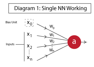
The different components are:
- x1, x2,…, xN: Inputs to the neuron. These can either be the actual observations from input layer or an intermediate value from one of the hidden layers.
- x0: Bias unit. This is a constant value added to the input of the activation function. It works similar to an intercept term and typically has +1 value.
- w0,w1, w2,…,wN: Weights on each input. Note that even bias unit has a weight.
- a: Output of the neuron which is calculated as:
Here f is known an activation function. This makes a Neural Network extremely flexible and imparts the capability to estimate complex non-linear relationships in data. It can be a gaussian function, logistic function, hyperbolic function or even a linear function in simple cases.
Lets implement 3 fundamental functions – OR, AND, NOT using Neural Networks. This will help us understand how they work. You can assume these to be like a classification problem where we’ll predict the output (0 or 1) for different combination of inputs.
We will model these like linear classifiers with the following activation function:
Example 1: AND
The AND function can be implemented as:
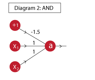
The output of this neuron is:
a = f( -1.5 + x1 + x2 )
The truth table for this implementation is:
Here we can see that the AND function is successfully implemented. Column ‘a’ complies with ‘X1 AND X2’. Note that here the bias unit weight is -1.5. But it’s not a fixed value. Intuitively, we can understand it as anything which makes the total value positive only when both x1 and x2 are positive. So any value between (-1,-2) would work.
Example 2: OR
The OR function can be implemented as:
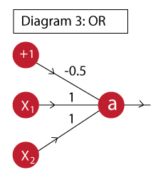
The output of this neuron is:
a = f( -0.5 + x1 + x2 )
The truth table for this implementation is:
Column ‘a’ complies with ‘X1 OR X2’. We can see that, just by changing the bias unit weight, we can implement an OR function. This is very similar to the one above. Intuitively, you can understand that here, the bias unit is such that the weighted sum will be positive if any of x1 or x2 becomes positive.
Example 3: NOT
Just like the previous cases, the NOT function can be implemented as:
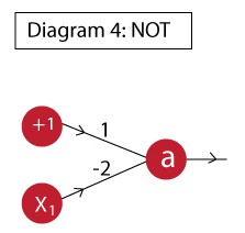
The output of this neuron is:
a = f( 1 – 2*x1 )
The truth table for this implementation is:
Again, the compliance with desired value proves functionality. I hope with these examples, you’re getting some intuition into how a neuron inside a Neural Network works. Here I have used a very simple activation function.
Note: Generally a logistic function will be used in place of what I used here because it is differentiable and makes determination of a gradient possible. There’s just 1 catch. And, that is, it outputs floating value and not exactly 0 or 1.
Why multi-layer networks are useful?
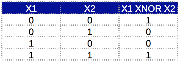
After understanding the working of a single neuron, lets try to understand how a Neural Network can model complex relations using multiple layers. To understand this further, we will take the example of an XNOR function. Just a recap, the truth table of an XNOR function looks like:
Here we can see that the output is 1 when both inputs are same, otherwise 0. This sort of a relationship cannot be modeled using a single neuron. (Don’t believe me? Give it a try!) Thus we will use a multi-layer network. The idea behind using multiple layers is that complex relations can be broken into simpler functions and combined.
Lets break down the XNOR function.
X1 XNOR X2 = NOT ( X1 XOR X2 )
= NOT [ (A+B).(A'+B') ] (Note: Here '+' means OR and '.' mean AND)
= (A+B)' + (A'+B')'
= (A'.B') + (A.B)
Now we can implement it using any of the simplified cases. I will show you how to implement this using 2 cases.
Case 1: X1 XNOR X2 = (A’.B’) + (A.B)
Here the challenge is to design a neuron to model A’.B’ . This can be easily modeled using the following:
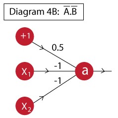
The output of this neuron is:
a = f( 0.5 – x1 – x2 )
The truth table for this function is:
Now that we have modeled the individual components and we can combine them using a multi-layer network. First, lets look at the semantic diagram of that network:
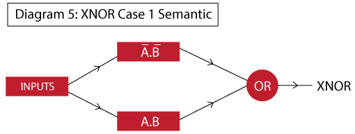
Here we can see that in layer 1, we will determine A’.B’ and A.B individually. In layer 2, we will take their output and implement an OR function on top. This would complete the entire Neural Network. The final network would look like this:
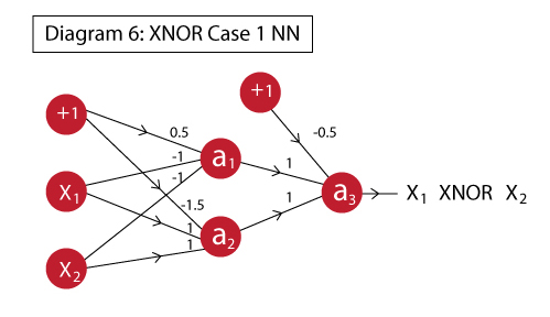
If you notice carefully, this is nothing but a combination of the different neurons which we have already drawn. The different outputs represent different units:
- a1: implements A’.B’
- a2: implements A.B
- a3: implements OR which works on a1 and a2, thus effectively (A’.B’ + A.B)
The functionality can be verified using the truth table:
I think now you can get some intuition into how multi-layers work. Lets do another implementation of the same case.
Case 2: X1 XNOR X2 = NOT [ (A+B).(A’+B’) ]
In the above example, we had to separately calculate A’.B’. What if we want to implement the function just using the basic AND, OR, NOT functions. Consider the following semantic:
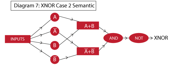
Here you can see that we had to use 3 hidden layers. The working will be similar to what we did before. The network looks like:
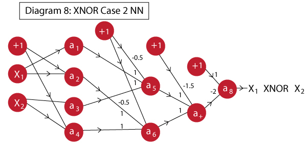
Here the neurons perform following actions:
- a1: same as A
- a2: implements A’
- a3: same as B
- a4: implements B’
- a5: implements OR, effectively A+B
- a6: implements OR, effectively A’+B’
- a7: implements AND, effectively (A+B).(A’+B’)
- a8: implements NOT, effectively NOT [ (A+B).(A’+B’) ] which is the final XNOR
Note that, typically a neuron feeds into every other neuron of the next layer except the bias unit. In this case, I’ve obviated few connections from layer 1 to layer 2. This is because their weights are 0 and adding them will make it visually cumbersome to grasp.
The truth table is:
Finally, we have successfully implemented XNOR function. This method is more complicated than case 1. Hence, you should prefer case 1 always. But the idea here is to show how complicated functions can be broken down in multiple layers. I hope the advantages of multiple layers are clearer now.
General Structure of a Neural Network
Now that we had a look at some basic examples, lets define a generic structure in which every Neural Network falls. We will also see the equations to be followed to determine the output given an input. This is known as Forward Propagation.
A generic Neural Network can be defined as:
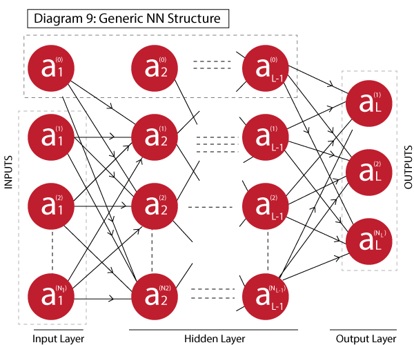
It has L layers with 1 input layer, 1 output layer and L-2 hidden layers. Terminology:
- L: number of layers
- Ni: number of neuron in ith layer excluding the bias unit, where i=1,2,…,L
- ai(j): the output of the jth neuron in ith layer, where i=1,2…L | j=0,1,2….Ni
Since the the output of each layer forms the input of next layer, lets define the equation to determine the output of i+1th layer using output of ith layer as input.
The input to the i+1th layer are:
Ai = [ ai(0), ai(1), ......, ai(Ni) ]
Dimension: 1 x Ni+1
The weights matrix from ith to i+1th layer is:
W(i) = [ [ W01(i)    W11(i)  .......   WNi1(i) ]
        [ W02(i)    W12(i)  .......   WNi2(i) ]
           ...                   ...
           ...                   ...
           ...                   ...
           ...                   ...
        [ W0Ni+1(i)  W1Ni+1(i)  ....... WNiNi+1(i) ] ]

Dimension: Ni+1 x Ni+1
The output of the i+1th layer can be calculated as:
 Ai+1 = f( Ai.W(i) )
Dimension: 1 x Ni+1
Using these equations for each subsequent layer, we can determine the final output. The number of neurons in the output layer will depend on the type of problem. It can be 1 for regression or binary classification problem or multiple for multi-class classification problems.
But this is just determining the output from 1 run. The ultimate objective is to update the weights of the model in order to minimize the loss function. The weights are updated using a back-propogation algorithm which we’ll study next.
Back-Propagation
Back-propagation (BP) algorithms works by determining the loss (or error) at the output and then propagating it back into the network. The weights are updated to minimize the error resulting from each neuron. I will not go in details of the algorithm but I will try to give you some intuition into how it works.
The first step in minimizing the error is to determine the gradient of each node wrt. the final output. Since, it is a multi-layer network, determining the gradient is not very straightforward.
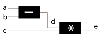
Let’s understand the gradients for multi-layer networks. Lets take a step back from neural networks and consider a very simple system as following:
Here there are 3 inputs which simple processing as:
d = a – b
e = d * c = (a-b)*c
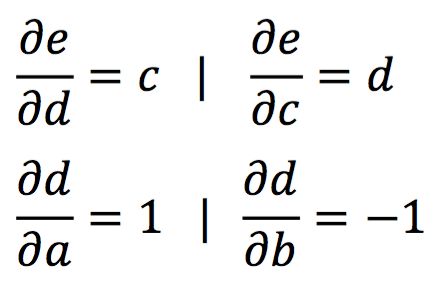
Now we need to determine the gradients of a,b,c,d wrt the output e. The following cases are very straight forward:
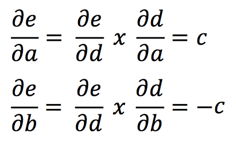
However, for determining the gradients for a and b, we need to apply the chain rule.
And, this way the gradient can be computed by simply multiplying the gradient of the input to a node with that of the output of that node. If you’re still confused, just read the equation carefully 5 times and you’ll get it!
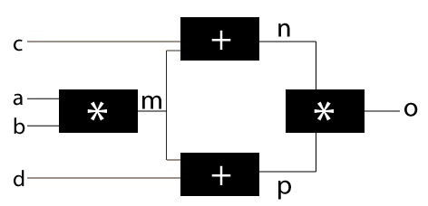
But, the actual cases are not that simple. Let’s take another example. Consider a case where a single input is being fed into multiple items in the next layer as this is almost always the case with neural network.
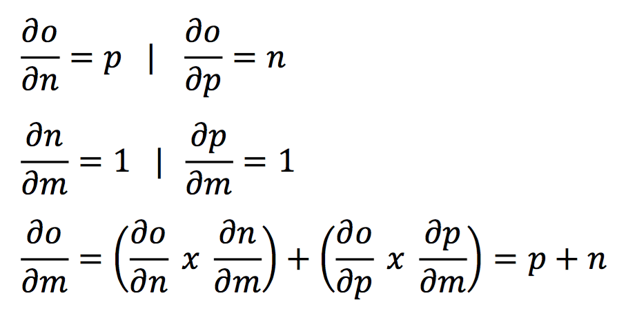
In this case, the gradients of all other will be very similar to the above example except for ‘m’ because m is being fed into 2 nodes. Here, I’ll show how to determine the gradient for m and rest you should calculate on your own.
Here you can see that the gradient is simply the summation of the two different gradients. I hope the cloud cover is slowly vanishing and things are becoming lucid. Just understand these concepts and we’ll come back to this.
Before moving forward, let’s sum up the entire process behind optimization of a neural network. The various steps involved in each iteration are:
- Select a network architecture, i.e. number of hidden layers, number of neurons in each layer and activation function
- Initialize weights randomly
- Use forward propagation to determine the output node
- Find the error of the model using the known labels
- Back-propogate the error into the network and determine the error for each node
- Update the weights to minimize gradient
Till now we have covered #1 – #3 and we have some intuition into #5. Now lets start from #4 – #6. We’ll use the same generic structure of NN as described in section 4.
#4- Find the error
eL(i) = y(i) - aL(i) | i = 1,2,....,NL
Here y(i) is the actual outcome from training data
#5- Back-propogating the error into the network
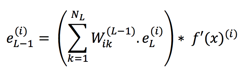
The error for layer L-1 should be determined first using the following:
where i = 0,1,2, ….., NL-1 (number of nodes in L-1th layer)
Intuition from the concepts discussed in former half of this section:
- We saw that the gradient of a node is a function of the gradients of all nodes from next layer. Here, the error at a node is based on weighted sum of errors on all the nodes of the next layer which take output of this node as input. Since errors are calculated using gradients of each node, the factor comes into picture.
- f'(x)(i) refers to the derivative of the activation function for the inputs coming into that node. Note that x refers to weighted sum of all inputs in present node before application of activation function.
- The chain rule is followed here by multiplication of the gradient of current node, i.e. f'(x)(i) with that of subsequent nodes which comes from first half of RHS of the equation.
This process has to be repeated consecutively from L-1th layer to 2nd layer. Note that the first layer is just the inputs.
#6- Update weights to minimize gradient
Use the following update rule for weights:
 Wik(l) = Wik(l) + a(i).el+1(k)
where,
- l = 1,2,….., (L-1) | index of layers (excluding the last layer)
- i = 0,1,….., Nl | index of node in lth layer
- k = 1,2,…., Nl+1 | index of node in l+1th layer
- Wik(l) refers to the weight from the lth layer to l+1th layer from ith node to kth node
I hope the convention is clear. I suggest you go through it multiple times and if still there are questions, I’ll be happy to take them on through comments below.
With this we have successfully understood how a neural network works. Please feel free to discuss further if needed.
Frequently Asked Questions
A. The fundamentals of deep learning include:
1. Neural Networks: Deep learning relies on artificial neural networks, which are composed of interconnected layers of artificial neurons.
2. Deep Layers: Deep learning models have multiple hidden layers, enabling them to learn hierarchical representations of data.
3. Training with Backpropagation: Deep learning models are trained using backpropagation, which adjusts the model’s weights based on the error calculated during forward and backward passes.
4. Activation Functions: Activation functions introduce non-linearity into the network, allowing it to learn complex patterns.
5. Large Datasets: Deep learning models require large labeled datasets to effectively learn and generalize from the data.
A. The fundamentals of neural networks include:
1. Neurons: Neural networks consist of interconnected artificial neurons that mimic the behavior of biological neurons.
2. Weights and Biases: Neurons have associated weights and biases that determine the strength of their connections and their activation thresholds.
3. Activation Function: Each neuron applies an activation function to its input, introducing non-linearity and enabling complex computations.
4. Layers: Neurons are organized into layers, including input, hidden, and output layers, which process and transform data.
5. Backpropagation: Neural networks are trained using backpropagation, adjusting weights based on error gradients to improve performance.
End Notes
This article is focused on the fundamentals of a Neural Network and how it works. I hope now you understand the working of a neural network and wouldn’t use it as a black box ever. It’s really easy once you understand doing it practically as well.
Therefore, in my upcoming article, I’ll explain the applications of using Neural Network in Python. More than theoretical, I’ll focus on practical aspect of Neural Network. Two applications come to my mind immediately:
- Image Processing
- Natural Language Processing
I hope you enjoyed this. I would love if you could share your feedback through comments below. Looking forward to interacting with you further on this!






Excellent Explanation , hope to see some practical example using R
I'll come up with examples when I have gained sufficient experience on this.
In some article, please explain convolution neural network and recursive neural network too.
Thanks for reaching out. I'll keep this in mind :)
Good one
Thanks!