Quick Guide to Build a Recommendation Engine in Python & R

Overview

• Deep dive into the concept of recommendation engine in python
• Building a recommendation system in python using the graphlab library
• Explanation of the different types of recommendation engines

Introduction

This could help you in building your first project!

Be it a fresher or an experienced professional in data science, doing voluntary projects always adds to one’s candidature. My sole reason behind writing this article is to get your started with recommendation systems so that you can build one. If you struggle to get open data, write to me in comments.

Recommendation engines are nothing but an automated form of a “shop counter guy”. You ask him for the product. Not only he shows that product, but also the related ones which you could buy. They are well trained in cross selling and up selling. So, does our recommendation engines.

The ability of these engines to recommend personalized content, based on past behavior is incredible. It brings customer delight and gives them a reason to keep returning to the website.

In this post, I will cover the fundamentals of creating a recommendation system using GraphLab in Python. We will get some intuition into how recommendation work and create basic popularity model and a collaborative filtering model.

Topics Covered

1. Type of Recommendation Engines
2. The MovieLens DataSet
3. A simple popularity model
4. A Collaborative Filtering Model
5. Evaluating Recommendation Engines

Before moving forward, I would like to extend my sincere gratitude to the Coursera’s Machine Learning Specialization by University of Washington. This course has been instrumental in my understanding of the concepts and this post is an illustration of my learnings from the same.

1. Type of Recommendation Engines

Before taking a look at the different types of recommendation engines, lets take a step back and see if we can make some intuitive recommendations. Consider the following cases:

Case 1: Recommend the most popular items

A simple approach could be to recommend the items which are liked by most number of users. This is a blazing fast and dirty approach and thus has a major drawback. The things is, there is no personalization involved with this approach.

Basically the most popular items would be same for each user since popularity is defined on the entire user pool. So everybody will see the same results. It sounds like, ‘a website recommends you to buy microwave just because it’s been liked by other users and doesn’t care if you are even interested in buying or not’.

Surprisingly, such approach still works in places like news portals. Whenever you login to say bbcnews, you’ll see a column of “Popular News” which is subdivided into sections and the most read articles of each sections are displayed. This approach can work in this case because:

• There is division by section so user can look at the section of his interest.
• At a time there are only a few hot topics and there is a high chance that a user wants to read the news which is being read by most others

Case 2: Using a classifier to make recommendation

We already know lots of classification algorithms. Let’s see how we can use the same technique to make recommendations. Classifiers are parametric solutions so we just need to define some parameters (features) of the user and the item. The outcome can be 1 if the user likes it or 0 otherwise. This might work out in some cases because of following advantages:

• Incorporates personalization
• It can work even if the user’s past history is short or not available

But has some major drawbacks as well because of which it is not used much in practice:

• The features might actually not be available or even if they are, they may not be sufficient to make a good classifier
• As the number of users and items grow, making a good classifier will become exponentially difficult

Case 3: Recommendation Algorithms

Now lets come to the special class of algorithms which are tailor-made for solving the recommendation problem. There are typically two types of algorithms – Content Based and Collaborative Filtering. You should refer to our previous article to get a complete sense of how they work. I’ll give a short recap here.

1. Content based algorithms:
   • Idea: If you like an item then you will also like a “similar” item
   • Based on similarity of the items being recommended
   • It generally works well when its easy to determine the context/properties of each item. For instance when we are recommending the same kind of item like a movie recommendation or song recommendation.
2. Collaborative filtering algorithms:
   • Idea: If a person A likes item 1, 2, 3 and B like 2,3,4 then they have similar interests and A should like item 4 and B should like item 1.
   • This algorithm is entirely based on the past behavior and not on the context. This makes it one of the most commonly used algorithm as it is not dependent on any additional information.
   • For instance: product recommendations by e-commerce player like Amazon and merchant recommendations by banks like American Express.
   • Further, there are several types of collaborative filtering algorithms :
     1. User-User Collaborative filtering: Here we find look alike customers (based on similarity) and offer products which first customer’s look alike has chosen in past. This algorithm is very effective but takes a lot of time and resources. It requires to compute every customer pair information which takes time. Therefore, for big base platforms, this algorithm is hard to implement without a very strong parallelizable system.
     2. Item-Item Collaborative filtering: It is quite similar to previous algorithm, but instead of finding customer look alike, we try finding item look alike. Once we have item look alike matrix, we can easily recommend alike items to customer who have purchased any item from the store. This algorithm is far less resource consuming than user-user collaborative filtering. Hence, for a new customer the algorithm takes far lesser time than user-user collaborate as we don’t need all similarity scores between customers. And with fixed number of products, product-product look alike matrix is fixed over time.
     3. Other simpler algorithms: There are other approaches like market basket analysis, which generally do not have high predictive power than the algorithms described above.

2. The MovieLens DataSet

We will be using the MovieLens dataset for this purpose. It has been collected by the GroupLens Research Project at the University of Minnesota. MovieLens 100K dataset can be downloaded from here. It consists of:

• 100,000 ratings (1-5) from 943 users on 1682 movies.
• Each user has rated at least 20 movies.
• Simple demographic info for the users (age, gender, occupation, zip)
• Genre information of movies

Lets load this data into Python. There are many files in the ml-100k.zip file which we can use. Lets load the three most importance files to get a sense of the data. I also recommend you to read the readme document which gives a lot of information about the difference files.

import pandas as pd

# pass in column names for each CSV and read them using pandas. 
# Column names available in the readme file

#Reading users file:
u_cols = ['user_id', 'age', 'sex', 'occupation', 'zip_code']
users = pd.read_csv('ml-100k/u.user', sep='|', names=u_cols,
 encoding='latin-1')

#Reading ratings file:
r_cols = ['user_id', 'movie_id', 'rating', 'unix_timestamp']
ratings = pd.read_csv('ml-100k/u.data', sep='\t', names=r_cols,
 encoding='latin-1')

#Reading items file:
i_cols = ['movie id', 'movie title' ,'release date','video release date', 'IMDb URL', 'unknown', 'Action', 'Adventure',
 'Animation', 'Children\'s', 'Comedy', 'Crime', 'Documentary', 'Drama', 'Fantasy',
 'Film-Noir', 'Horror', 'Musical', 'Mystery', 'Romance', 'Sci-Fi', 'Thriller', 'War', 'Western']
items = pd.read_csv('ml-100k/u.item', sep='|', names=i_cols,
 encoding='latin-1')

print(users.shape)
print(users.head())

Now lets take a peak into the content of each file to understand them better.

• 
  

  Users

  
  

print users.shape
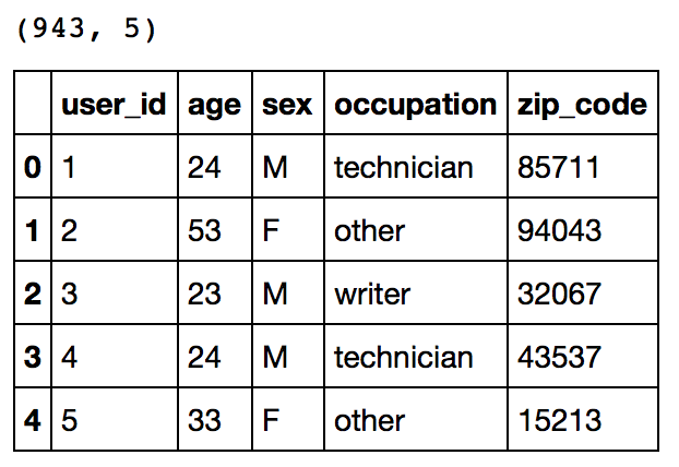
users.head()

This reconfirms that there are 943 users and we have 5 features for each namely their unique ID, age, gender, occupation and the zip code they are living in.

• 
  

  Ratings

  
  

print ratings.shape
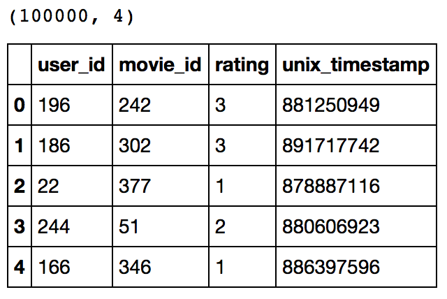
ratings.head()

This confirms that there are 100K ratings for different user and movie combinations. Also notice that each rating has a timestamp associated with it.

• 
  

  Items

  
  

print items.shape
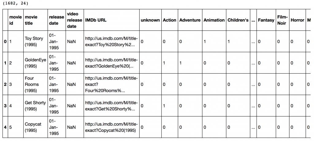
items.head()

This dataset contains attributes of the 1682 movies. There are 24 columns out of which 19 specify the genre of a particular movie. The last 19 columns are for each genre and a value of 1 denotes movie belongs to that genre and 0 otherwise.

Now we have to divide the ratings data set into test and train data for making models. Luckily GroupLens provides pre-divided data wherein the test data has 10 ratings for each user, i.e. 9430 rows in total. Lets load that:

r_cols = ['user_id', 'movie_id', 'rating', 'unix_timestamp']
ratings_base = pd.read_csv('ml-100k/ua.base', sep='\t', names=r_cols, encoding='latin-1')
ratings_test = pd.read_csv('ml-100k/ua.test', sep='\t', names=r_cols, encoding='latin-1')
ratings_base.shape, ratings_test.shape

Output: ((90570, 4), (9430, 4))

Since we’ll be using GraphLab, lets convert these in SFrames.

import graphlab
train_data = graphlab.SFrame(ratings_base)
test_data = graphlab.SFrame(ratings_test)

We can use this data for training and testing. Now that we have gathered all the data available. Note that here we have user behaviour as well as attributes of the users and movies. So we can make content based as well as collaborative filtering algorithms.

3. A Simple Popularity Model

Lets start with making a popularity based model, i.e. the one where all the users have same recommendation based on the most popular choices. We’ll use the  graphlab recommender functions popularity_recommender for this.

We can train a recommendation as:

popularity_model = graphlab.popularity_recommender.create(train_data, user_id='user_id', item_id='movie_id', target='rating')

Arguments:

• train_data: the SFrame which contains the required data
• user_id: the column name which represents each user ID
• item_id: the column name which represents each item to be recommended
• target: the column name representing scores/ratings given by the user

Lets use this model to make top 5 recommendations for first 5 users and see what comes out:

#Get recommendations for first 5 users and print them
#users = range(1,6) specifies user ID of first 5 users
#k=5 specifies top 5 recommendations to be given
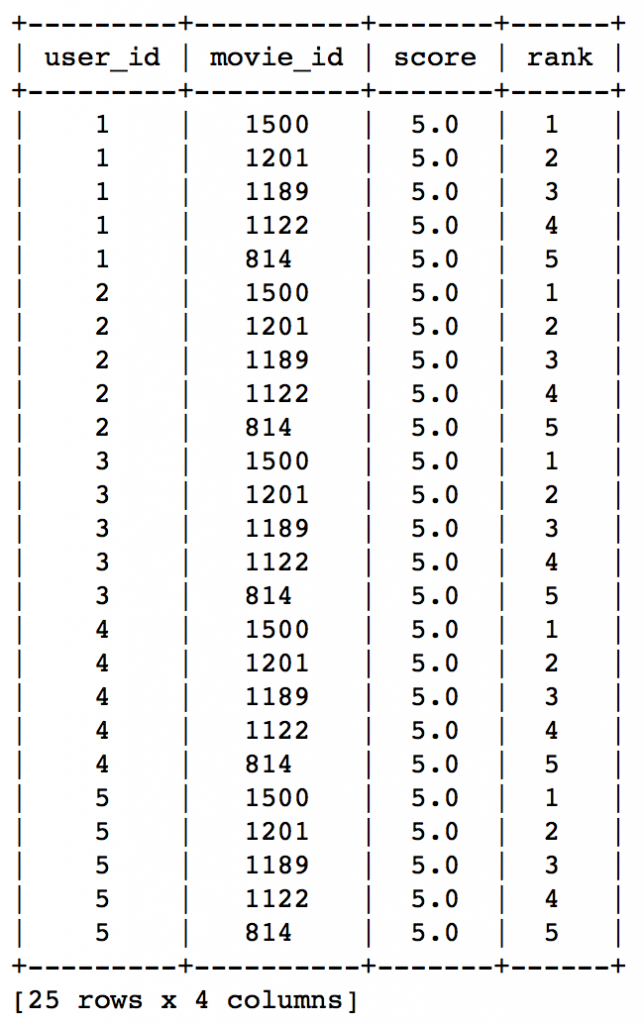
popularity_recomm = popularity_model.recommend(users=range(1,6),k=5)
popularity_recomm.print_rows(num_rows=25)

Did you notice something? The recommendations for all users are same – 1500,1201,1189,1122,814 in the same order. This can be verified by checking the movies with highest mean recommendations in our ratings_base data set:

ratings_base.groupby(by='movie_id')['rating'].mean().sort_values(ascending=False).head(20)

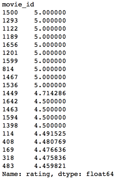
This confirms that all the recommended movies have an average rating of 5, i.e. all the users who watched the movie gave a top rating. Thus we can see that our popularity system works as expected. But it is good enough? We’ll analyze it in detail later.

4. A Collaborative Filtering Model

Lets start by understanding the basics of a collaborative filtering algorithm. The core idea works in 2 steps:

1. Find similar items by using a similarity metric
2. For a user, recommend the items most similar to the items (s)he already likes

To give you a high level overview, this is done by making an item-item matrix in which we keep a record of the pair of items which were rated together.

In this case, an item is a movie. Once we have the matrix, we use it to determine the best recommendations for a user based on the movies he has already rated. Note that there a few more things to take care in actual implementation which would require deeper mathematical introspection, which I’ll skip for now.

I would just like to mention that there are 3 types of item similarity metrics supported by graphlab. These are:

1. Jaccard Similarity: 
   • Similarity is based on the number of users which have rated item A and B divided by the number of users who have rated either A or B
   • It is typically used where we don’t have a numeric rating but just a boolean value like a product being bought or an add being clicked
2. Cosine Similarity:
   • Similarity is the cosine of the angle between the 2 vectors of the item vectors of A and B
   • Closer the vectors, smaller will be the angle and larger the cosine
3. Pearson Similarity
   • Similarity is the pearson coefficient between the two vectors.

Lets create a model based on item similarity as follow:

#Train Model
item_sim_model = graphlab.item_similarity_recommender.create(train_data, user_id='user_id', item_id='movie_id', target='rating', similarity_type='pearson')

#Make Recommendations:
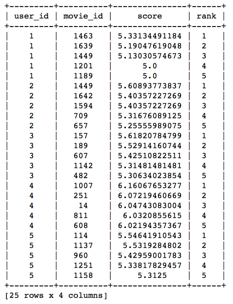
item_sim_recomm = item_sim_model.recommend(users=range(1,6),k=5)
item_sim_recomm.print_rows(num_rows=25)

Here we can see that the recommendations are different for each user. So, personalization exists. But how good is this model? We need some means of evaluating a recommendation engine. Lets focus on that in the next section.

5. Evaluating Recommendation Engines

For evaluating recommendation engines, we can use the concept of precision-recall. You must be familiar with this in terms of classification and the idea is very similar. Let me define them in terms of recommendations.

• Recall:
  • What ratio of items that a user likes were actually recommended.
  • If a user likes say 5 items and the recommendation decided to show 3 of them, then the recall is 0.6
• Precision
  • Out of all the recommended items, how many the user actually liked?
  • If 5 items were recommended to the user out of which he liked say 4 of them, then precision is 0.8

Now if we think about recall, how can we maximize it? If we simply recommend all the items, they will definitely cover the items which the user likes. So we have 100% recall! But think about precision for a second. If we recommend say 1000 items and user like only say 10 of them then precision is 0.1%. This is really low. Our aim is to maximize both precision and recall.

An idea recommender system is the one which only recommends the items which user likes. So in this case precision=recall=1. This is an optimal recommender and we should try and get as close as possible.

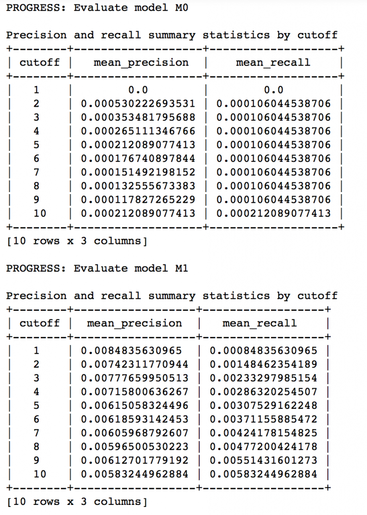
Lets compare both the models we have built till now based on precision-recall characteristics:

model_performance = graphlab.compare(test_data, [popularity_model, item_sim_model])
graphlab.show_comparison(model_performance,[popularity_model, item_sim_model])

Here we can make 2 very quick observations:

1. The item similarity model is definitely better than the popularity model (by atleast 10x)
2. On an absolute level, even the item similarity model appears to have a poor performance. It is far from being a useful recommendation system.

Now let us learn to build a recommendation engine in R

Implementation in R

Step 1: Importing the data files 

Step 2: Validating the imported data files

Output

#Validating user files

[1] 943 5

user_id age sex occupation zip_code
1 1 24 M technician 85711
2 2 53 F other 94043
3 3 23 M writer 32067
4 4 24 M technician 43537
5 5 33 F other 15213
6 6 42 M executive 98101

#Validating ratings files

[1] 100000 4

user_id movie_id rating unix_timestamp
1 196 242 3 881250949
2 186 302 3 891717742
3 22 377 1 878887116
4 244 51 2 880606923
5 166 346 1 886397596
6 298 474 4 884182806

#Validating items files

[1] 1682 24

Step 3: Loading the train and test dataset

Step 4: Validating the test and train dataset

Output

#Validating train files

[1] 90570 4

user_id movie_id rating unix_timestamp
1 1 1 5 874965758
2 1 2 3 876893171
3 1 3 4 878542960
4 1 4 3 876893119
5 1 5 3 889751712
6 1 6 5 887431973

 #Validating test files

[1] 9430 4

user_id movie_id rating unix_timestamp
1 1 20 4 887431883
2 1 33 4 878542699
3 1 61 4 878542420
4 1 117 3 874965739
5 1 155 2 878542201
6 1 160 4 875072547

Step 5 Building a simple Popularity Model

The movies with the highest mean recommendations in our data_train data set:

Output

 movie_id rating

814 5.000000
1122 5.000000
1189 5.000000
1201 5.000000
1293 5.000000
1467 5.000000
1500 5.000000
1536 5.000000
1599 5.000000
1656 5.000000
1449 4.714286
1398 4.500000
1463 4.500000
1594 4.500000
1642 4.500000
114 4.491525
408 4.480769
169 4.476636
318 4.475836
483 4.459821

All the recommended movies have an average rating of 5, i.e. all the users who watched the movie gave a top rating. Thus we can see that our popularity system works as expected.

Step 6 Building a collaborating filtering model

Let’s create a model based on item similarity as follow:

model1
Recommender of type ‘IBCF’ for ‘binaryRatingMatrix’ 
learned using 90570 users.

predicted1
Recommendations as ‘topNList’ with n = 10 for 9430 users. 

head(reccom_list,25)
user_id rating movie_id
1 0.5085274 10
1 0.5000725 5
1 0.5035601 3
1 0.5051816 3
1 0.5121527 4
1 0.5000000 8
1 0.5009827 2
1 0.5035601 12
2 0.5036726 3
2 0.5000000 3
2 0.5017065 2
2 0.5019525 5
2 0.5060604 11
2 0.5000000 12
2 0.5002561 7
2 0.5016215 8
3 0.5014799 5
3 0.5124669 4
3 0.5014799 5
3 0.5009827 9
3 0.5052220 1
3 0.5060604 11
3 0.5000000 6
3 0.5009737 1
4 0.5014341 6

Here we can see that the recommendations are different for each user. So, personalization exists. But how good is this model? We need some means of evaluating a recommendation engine. Let’s focus on that in the next section.

Step 7 – Evaluating Recommendation Engines

Let’s compare both the models we have built till now based on precision-recall characteristics:

Observations

1. The item similarity model is definitely better than the popularity model (by at least 10x)
2. On an absolute level, even the item similarity model appears to have a poor performance. It is far from being a useful recommendation system.

There is a big scope of improvement here. But I leave it up to you to figure out how to improve this further. I would like to give a couple of tips:

1. Try leveraging the additional context information which we have
2. Explore more sophisticated algorithms like matrix factorization

In the end, I would like to mention that along with GraphLab, you can also use some other open source python packages like the following:

• Crab.
• Surprise
• Python Recsys
• MRec

Projects

Now, its time to take the plunge and actually play with some other real datasets. So are you ready to take on the challenge? Accelerate your journey and use recommendation engines to solve these Practice Problems:

	Online Challenge: Build A Recommendation Engine	Recommend the next items customers are most likely to buy
	Practice Problem: Recommendation Engine	Predict range of attempts a user will make to solve a given problem
	Practice Problem: Is this joke funny?	Predict the rating given by users to different jokes

End Notes

In this article, we traversed through the process of making a basic recommendation engine in Python using GrpahLab. We started by understanding the fundamentals of recommendations. Then we went on to load the MovieLens 100K data set for the purpose of experimentation.

Subsequently we made a first model as a simple popularity model in which the most popular movies were recommended for each user. Since this lacked personalization, we made another model based on collaborative filtering and observed the impact of personalization.

Finally, we discussed precision-recall as evaluation metrics for recommendation systems and on comparison found the collaborative filtering model to be more than 10x better than the popularity model.

Did you like reading this article ?  Do share your experience / suggestions in the comments section below.

You can test your skills and knowledge. Check out Live Competitions and compete with best Data Scientists from all over the world.

Aarshay Jain

Aarshay graduated from MS in Data Science at Columbia University in 2017 and is currently an ML Engineer at Spotify New York. He works at an intersection or applied research and engineering while designing ML solutions to move product metrics in the required direction. He specializes in designing ML system architecture, developing offline models and deploying them in production for both batch and real time prediction use cases.