A Beginner’s guide to Shelf Space Optimization using Linear Programming

Introduction

Have you ever wondered why products in a Retail Store are placed in a certain manner? In the world of analytics, where retail giants like Walmart, Target etc. are collecting terabytes of data on a daily basis, every decision in the brick and mortar stores is carefully thought through and analyzed. Further, with an increasing number of smart shopping outlets, the data collection and the level of analysis have both become far more granular.

Shelf space maximisation is one of key factors behind any marketing strategy for a brand. In this article, I will explain some challenges in shelf space optimization and then solve a toy example using excel, python and greedy algorithm. Read on to find detailed description along with the codes.

Table of Contents

• The Basic Concepts
  • Optimization
  • Linear Programming
• Shelf Space Optimization and its challenges
• Defining & Solving the Problem
  • Linear Optimization using Excel
  • Linear Optimization using Pulp library in Python
  • Greedy Algorithm
• Challenges with large Datasets
• Conclusion and LP examples

Let me start by introducing the concepts we would be using later on:

The basic concepts

In this section, I’ll introduce some terms I’ll be using later in the article.

Optimization

Optimization is the science / process behind finding the best solution for a problem with given constraints. We come across optimization problems on a daily basis. These can be for finding the shortest path between your work place and office; maximizing revenues / customer happiness or minimizing costs / debts etc. We basically take a real world problem, model it mathematically and then solve it using mathematical techniques with in the constraints. Optimization is useful in Marketing, Manufacturing, Finance, Online advertising, Machine Learning and all fields you can imagine.

Linear Programming

Linear programming (LP) (also called linear optimization) is a method to achieve the best outcome (such as maximum profit or lowest cost) in a mathematical model whose requirements are represented by linear relationships. Linear programs can be expressed by:

1. Decision Variables
2. An Objective function: Must be linear
3. Constraints: Must be linear equalities or inequalities.

A linear programming algorithm finds a point in the feasible space where the Objective function has the smallest (or largest) value if such a point exists. Simplex Algorithm is the most commonly used algorithm to solve Linear Programming.

Integer Programming is a special case of Linear Programming where the decision variables are restricted to be Integers. We will deal with an Integer Programming problem with only binary 0-1 outcomes.

Shelf Space Optimization

In a store, a product’s position in store can greatly affect its performance. Having the right space allocation for products and categories plays a critical role in its retail success. From retailers perspective, given the value of shelf space positions, it is very critical to ensure that retail space is working for value maximization for the store.

The shelves near the POS offer maximum visibility to the customers and help the stores reap in those extra few dollars for items which were not even in the shoppers list. Marketing the right merchandise, at the right place, at the right time, in the right quantities is key to retail revenues and profitability. This has led to a war between brands to occupy the best possible space in a store. On the other hand, the stores also have to optimize their overall profitability considering the sales of all merchandise.

Challenges

The logic is comprehensible, but applying it can be difficult because the information needed for Space Optimization is most times unclear, complex or scattered throughout the business. Certain products may play a vital role (being essential to promotions program for instance); others may be duplicates / clones, but provide higher margins etc. Hence it may become difficult to measure them on a single parameter. Besides, an average retailer stocks around 30,000 SKU’s (different products). Thousands of new items are introduced at retail every year. Optimizing a problem of that size becomes extremely difficult and often requires SME’s, Consultants and Statisticians to brainstorm a lot.

Defining the Problem & solving it

This is a toy problem but the same concept can be expanded for a problem of bigger size. Let us understand the problem.

Lifts Table

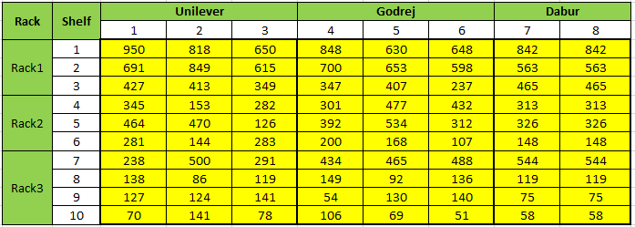
Let us assume a retail store with 3 racks, Rack 1, Rack2 and Rack3 with 3, 3 and 4 shelves as shown in the below table. We have to stock products of 3 companies Unilever, Godrej and Dabur. Unilever, Godrej and Dabur has 3, 3 and 2 products respectively. The numbers that we see in the matrix are the lifts (increase in sales) that we achieve on placing a specific product on a specific rack / shelf (given by corresponding row).

Now due to a difference in profit margin / inventory cost / demand / expiration date etc. of products, the store wants to optimize the placement of each product on the shelves and maximize the total sales (number of products) taking into account the constraints it has got.

Decision Variables

The decision variables will be in the form of a matrix of the same size as lift (10*8). The matrix will have binary values, 1 indicating a YES for the product/shelf pair and 0 indicating a NO. We will start with a matrix of all 0’s and allow the solver to make changes to 1’s where required.

Objective Function

The objective function to be maximized is the Total Sales of all merchandize.

Constraints

The constraints used here are:

1. One Shelf can have at max one product of any company.(row constraint)
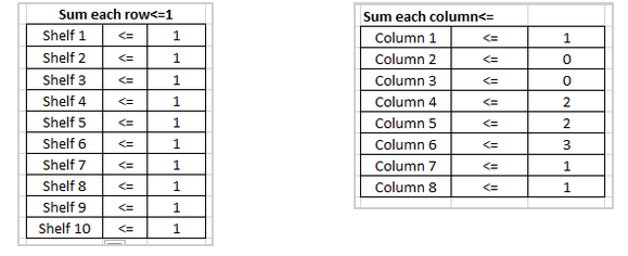
2. The products cannot be marketed more than a particular number of times. This is given in the order of the products as shown in above fig. (Column constraint). The maximum occurrences of the products are as below. These constraints can be attributed to the product type/profit margin/demand or any other rationale applicable at the store.

This boils down to the conditions that Product 1 from Unilever cannot be marketed more than once. Similarly for the other products the constraints apply.

There can be several more constraints applied as per the business understanding of a store and merchandizing best practices. However for this learning problem, this would suffice.

Linear Optimization using Excel

Constraints can be taken care using the above two tables in excel.

1. Constraint 1 will always be satisfied when the sum of the rows<=1
2. Constraint 2 will always hold true when the sum of each column<=the list of the column constraints as shown before.

Let us go to the Solver in Excel. Go to DATA → Solver. If it’s not visible you need to activate it by going to File → Options → Add-Ins

This is how it looks like.

Set Objective

The Objective function is given by the sumproduct of the lift and the decision variable matrix. Select the cell in spreadsheet which indicates this.

We have to maximize the Profit.

Decision variable is the matrix of same size as the lift. Select all cells representing it.

For constraints select the cells that represent the Sum of rows and Sum of columns in the decision variable matrix. Assign them <= inequality. For all rows the sum <=1 and for columns it is given by the list of constraints as given in problem.

Add another constraint to make the decision variables binary integers. (0’s and 1’s).

Select Simplex LP and run.

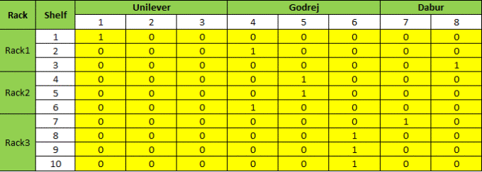
The objective function along with the constraints is solved and the maximum sales obtained is 4197. The decision variable matrix obtained is shown below:

That was easy. But Excel has its limitations and cannot be used for a problems of large size. Also if there are too many constraints it will be a humongous task to take that in excel. That’s where Python comes to the rescue.

Linear Optimization using Pulp library in Python

Spreadsheet optimization is too cumbersome to use for day to day operation. Python can easily be used for large problem size and will only be limited by the computing limitations. Also once coded / automated it can be run for problems of varying sizes. Any new constraints can also be taken care later as and when they arise. I use Pulp library in python and its open source solver CBC to arrive at the best possible solution. There are other commercial solvers available like CPLEX, GUROBI etc. which are useful for very large problems as they provide speedier / better results.

The python codes for as follows:

#import all relevant libraries

import pandas as pd

import numpy as np

import math

from math import isnan

from pulp import *

from collections import Counter

from more_itertools import unique_everseen

sales=pd.read_csv("sales_lift.csv",header=None) #input file

lift=sales.iloc[2:,1:]

lift=np.array(lift)

lift = lift.astype(np.int) # read the lifts from csv

brands=sales.iloc[0:1,:]

brands=np.array(brands)

brands=np.delete(brands,0)

brands=brands.tolist()  # read the brands from csv

ff=Counter(brands)

all_brands=ff.items()

# the racks and the shelfs available

rack_shelf=[[1,1,2,3],[2,4,5,6],[3,7,8,9,10]]

#define the optimization function

prob=LpProblem("SO",LpMaximize)

#define decision variables

dec_var=LpVariable.matrix("dec_var",(range(len(lift)),range(len(lift[0]))),0,1,LpBinary)

#Compute the sum product of decision variables and lifts

prodt_matrix=[dec_var[i][j]*lift[i][j] for i in range(len(lift))

for j in range(len(lift[0]))]

#total lift which has to be maximized sum(prodt_matrix)

#define the objective function

prob+=lpSum(prodt_matrix)

order=list(unique_everseen(brands))

order_map = {}

for pos, item in enumerate(order):

    order_map[item] = pos

#brands in order as in input file

brands_lift=sorted(all_brands, key=lambda x: order_map[x[0]])

DEFINE CONSTRAINTS

1) Each shelf can have only one product i.e. sum (each row)<=1

for i in range(len(lift)):

    prob+=lpSum(dec_var[i])<=1

2) Each product can be displayed only on a limited number of shelves i.e. Column constraints

Constraints are given as

col_con=[1,0,0,2,2,3,1,1]

dec_var=np.array(dec_var)

col_data=[]

for j in range(len(brands)):

    col_data.append(list(zip(*dec_var)[j]))

    prob+=lpSum(col_data[j])<=col_con[j]

#write the problem

prob.writeLP("SO.lp")

#solve the problem

prob.solve()

print("The maximum Total lift obtained is:",value(prob.objective)) # print the output

#print the decision variable output matrix

Matrix=[[0 for X in range(len(lift[0]))] for y in range(len(lift))]

for v in prob.variables():

    Matrix[int(v.name.split("_")[2])][int(v.name.split("_")[3])]=v.varValue

    matrix=np.int_(Matrix)

print ("The decision variable matrix is:")

print(matrix)

The results from python and Excel match exactly. This reinforces that the result obtained is the global maximum (lift), 4197 as the Total Lift.

Challenges with Large Datasets

Let us understand what problems arise with large datasets. As in this example we understand that each decision variable can take values 0 or 1 that is 2^1 or 2 possible values. For 2 decision variables the total number of possible combinations can be 2^2 or 4 out of which one/more may give the optimized value of the Objective function. With 80 decision variables in our example, the total combinations is 2^80. This shows that the order of the problem is exponential and not linear. [In language of Computational Complexity Theory, exponential time O (2^n)]. Problems of exponential order are very intensive even for the best of computers. As in our example each of the 2^80 combinations will be evaluated to find the optimized solution.

That’s where business understanding and domain knowledge comes into picture. A SME should be able to quickly reject some of the combinations by applying appropriate constraints to the problem and hence limiting the total # of possible solutions.

Greedy Algorithm

Let us see how a greedy algorithm would perform under the same constraints. A greedy algorithm, as the name suggests tries to maximize the lift in each step irrespective of the total gain. This may or may not (in most cases) give the global optimum. Our greedy algorithm will attack the problem in the following way:

1. Find the maximum lift in the entire lift matrix. Say it comes at index: lifts[i, j].
2. Check for the constraints in the decision variable matrix (dec_var) for row i and column j.
3. If all constraints are satisfied, change the value of dec_var[i, j] =1.
4. Since there can be only one 1 in a row, make all remaining elements of row i as 0.
5. If constraints are not satisfied, again make all elements of the row 0
6. Repeat 1 to 5.

Other applications of optimization problems

Now that you have seen a basic implementation of an optimization problem, let us understand applications in a few other domains:

Google AdWords: Google uses LP for its online advertising. Google has different slots on its search page and based on the PPC (price per click), CTR (Click through Rate) and Budget (constraint) of the advertisers Google allots the slots and the number of times (decision variables) to display the add while maximizing its revenue (objective function). AdWords account for ~97% of Google’s revenue.

Airlines Revenue Management: Airlines use linear optimization to offer limited discounted tickets (decision variable) and also maximize their revenues (objective) for a forecasted demand (constraint) and plane type (limited seats, also constraints).

Cancer treatment: LP is used to treat cancer patients by radiation. Tumorous cells are targeted with a desired radiation level (constraint) and at the same time the healthy tissue should be exposed to least radiation (minimize objective function).

Promotion of ads on Television Channels: A TV channel has tens of Shows and thousands of promotions and commercials to market. Through linear optimization they decide which promotion to telecast in which slot and maintain a high audience viewership (Objective). Constraints come in the form of Budget of each promotions, max number of times a promotion can be shown etc.

Dating Sites: Linear Optimization is also used by online dating sites like eHarmony. Based on a questionnaire which each user fills, eHarmony computes a compatibility score between two people and uses optimization algorithms like Linear Programming to determine their users’ best matches. Possible constraints here are Men are matched to only Women; One Man is matched to one Woman and vice versa.

Conclusion

The toy problem can be expanded into a problem for the entire store where there would be thousands of Racks/Shelves etc. The constraints will also accordingly increase to thousands. This will allow the store to place an item at the right place and derive maximum total sales.

End Notes

 I hope this will be a good reference material for beginners in Optimization. I am also in the process of exploring this further and doing more complex problems on it. LP has been an inherent part of Operations and Inventory management and many organizations have their own in-house tools for it. I hope you enjoyed reading this article and found it helpful. I would love to hear from you, if you have any questions / feedback / doubts feel free to drop in your comments below.

About the Author

Deepesh Singh is a Data Science enthusiast. He is a continuous learner and loves exploring diverse areas of Data Science. An engineer from NIT Silchar and armed with a one year certificate in Business Analytics from IIM-L and KSB (Indiana University), he currently solves business problems at Bangalore office of an Analytics organization. Outside of work, he loves Toast-mastering, working out at gym, practicing/teaching karate.

Got expertise in Business Intelligence  / Machine Learning / Big Data / Data Science? Showcase your knowledge and help Analytics Vidhya community by posting your blog.