Introduction
We have seen the in-depth detailed implementation of neural networks in Keras and Theano in the previous articles. I think both the libraries are fascinating with their pros one over the other. I decided to make this more interesting and do a comparison between two superpowers of Deep Learning.
In this article, I’ve covered a basic overview of Keras and Theano. Then I will be explaining in details with the help of use cases why & when should one prefer Theano over Keras. Then I’ve explained about advanced techniques like transfer learning and fine tuning, with a case study combining all the mentioned topics.
Note:
- This article is best suited for users with clear understanding neural networks, deep learning, keras & theano.
- If you are not well equipped with Deep Learning, read here.
- If you are not familiar with Keras, read here.
- If you are not familiar with Theano, read here.
Table of Contents
- A bit about the superpowers
- When should you prefer Theano over Keras?
- Simple neural network model using Theano
- Getting to know Transfer Learning and Fine tuning
- Case study with Keras and Theano
- Where to go from here?
- Additional Resources
A bit about the superpowers
Before we proceed further, let’s look at the definitions of Theano and Keras.
Theano in a few lines:
A programming language which runs on top of Python but has its own data structure which are tightly integrated with numpy, allowing faster implementation of mathematical expressions
Keras in a few lines:
Keras is a high level library, used specially for building neural network models. Keras was specifically developed for fast execution of ideas. It is written in (and for) Python
Theano and Keras are built keeping specific things in mind and they excel in the fields they were built for. Theano is more of a matrix manipulation library with an optimized compiler on its backend. Whereas Keras is a deep learning library built over Theano to abstract most of the code to give an easier interface.
When would you prefer Theano over Keras?
Keras is a very useful deep learning library but it has its own pros and cons, which has been explained in my previos article on Keras. The main scenario in which you would prefer Theano is when you want to build a custom neural network model.
Theano is flexible enough when it comes to building your own models. You can write you own functions and optimizations and easily integrate it with your model. This is especially useful in research environment, when it comes to innovating new ideas.
Let’s take an example:
A recently published paper called “Binarized Neural Networks: Training Neural Networks with Weights and Activations Constrained to +1 or −1” uses an innovative strategy. As the name says, they change the typical values of weights & activations and replace them with binary values.
To build this “Binary Net”, you would have to rewrite the code for value representations in a neural network. So using low-level libraries like Theano, can easily make this possible.
Simple neural network model using Theano
Now, I will be taking you through an implementation of a neural network written in Theano.
A typical implementation of Neural Network would be as follows:
- Define Neural Network architecture to be compiled
- Transfer data to your model
- Under the hood, the data is first divided into batches, so that it can be ingested. The batches are first preprocessed, augmented and then fed into Neural Network for training
- The model then gets trained incrementally
- Display the accuracy for a specific number of timesteps
- After training save the model for future use
- Test the model on a new data and check how it performs
Here we solve our deep learning practice problem – Identify the Digits. Let’s for a moment take a look at our problem statement.
Our problem is an image recognition, to identify digits from a given 28 x 28 image. We have a subset of images for training and the rest for testing our model. So first, download the train and test files. The dataset contains a zipped file of all the images in the dataset and both the train.csv and test.csv have the name of the corresponding train and test images. Any additional features are not provided in the datasets, just the raw images are provided in ‘.png’ format.
Now let’s first get to know how to build a neural network model in Theano.
- Let’s import all the required modules
%pylab inline

import os
import numpy as np
import pandas as pd
from scipy.misc import imread
from sklearn.metrics import accuracy_score

import theano
import theano.tensor as T
- Let’s set a seed value, so that we can control our model’s randomness
# To stop potential randomness
seed = 128
rng = np.random.RandomState(seed)
- The first step is to set directory paths for safekeeping!
root_dir = os.path.abspath('../..')
data_dir = os.path.join(root_dir, 'data')
sub_dir = os.path.join(root_dir, 'sub')

# check for existence
os.path.exists(root_dir)
os.path.exists(data_dir)
- Now let us read our datasets. These are in .csv format, and have a filename along with the appropriate labels
train = pd.read_csv(os.path.join(data_dir, 'Train', 'train.csv'))
test = pd.read_csv(os.path.join(data_dir, 'Test.csv'))

sample_submission = pd.read_csv(os.path.join(data_dir, 'Sample_Submission.csv'))
| filename | label | |
|---|---|---|
| 0 | 0.png | 4 |
| 1 | 1.png | 9 |
| 2 | 2.png | 1 |
| 3 | 3.png | 7 |
| 4 | 4.png | 3 |
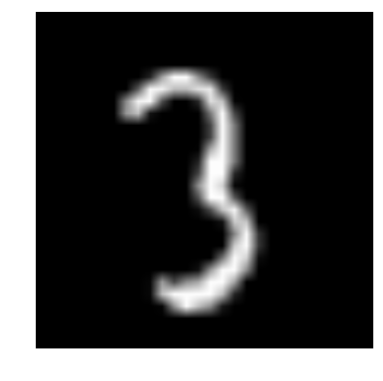
- Let us see what our data looks like! We read our image and display it.
img_name = rng.choice(train.filename)
filepath = os.path.join(data_dir, 'Train', 'Images', 'train', img_name)

img = imread(filepath, flatten=True)

pylab.imshow(img, cmap='gray')
pylab.axis('off')
pylab.show()
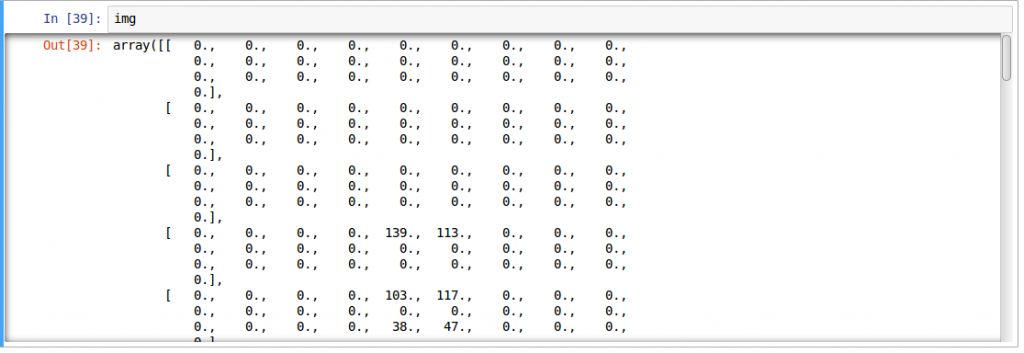
The above image is represented as numpy array, as seen below:
- For easier data manipulation, let’s store all our images as numpy arrays
temp = []
for img_name in train.filename:
 image_path = os.path.join(data_dir, 'Train', 'Images', 'train', img_name)
 img = imread(image_path, flatten=True)
 img = img.astype('float32')
 temp.append(img)

train_x = np.stack(temp)

temp = []
for img_name in test.filename:
 image_path = os.path.join(data_dir, 'Train', 'Images', 'test', img_name)
 img = imread(image_path, flatten=True)
 img = img.astype('float32')
 temp.append(img)

test_x = np.stack(temp)
- As this is a typical ML problem, to test the proper functioning of our model we create a validation set. Let’s take a split size of 70:30 for train set vs validation set.
split_size = int(train_x.shape[0]*0.7)

train_x, val_x = train_x[:split_size], train_x[split_size:]
train_y, val_y = train.label.values[:split_size], train.label.values[split_size:]
train_x = train_x.reshape(-1, 784)
val_x = val_x.reshape(-1, 784)
test_x = test_x.reshape(-1, 784)
- Now we define some helper functions, which we use later on, in our program
def dense_to_one_hot(labels_dense, num_classes=10):
    """Convert class labels from scalars to one-hot vectors"""
    num_labels = labels_dense.shape[0]
    index_offset = numpy.arange(num_labels) * num_classes
    labels_one_hot = numpy.zeros((num_labels, num_classes))
    labels_one_hot.flat[index_offset + labels_dense.ravel()] = 1

    return labels_one_hot

def preproc(unclean_batch_x):
    """
    Convert values to range 0-1
    """
    temp_batch = unclean_batch_x / unclean_batch_x.max()

   return temp_batch

def batch_creator(batch_size, dataset_x, dataset_y):
    """
    Create batch with random samples
    """
    batch_mask = rng.choice(dataset_x.shape[0], batch_size)

    batch_x = dataset_x[batch_mask]
    batch_y = dataset_y[batch_mask]

    batch_x = preproc(batch_x)
    batch_y = dense_to_one_hot(batch_y)

    return batch_x, batch_y

def to_theano_float(arr):
    """Convert numpy array to theano tensors"""
    return np.asarray(arr, dtype=theano.config.floatX)
- Now comes the main part! Let us define our neural network architecture. We define a neural network with 3 layers input, hidden and output. The number of neurons in input and output are fixed, as the input is our 28 x 28 image and the output is a 10 x 1 vector representing the class. We take 500 neurons in the hidden layer. This number can vary according to your need. We also assign values to remaining variables. Read the article on fundamentals of neural network to know more in depth of how it works.
# number of neurons in each layer
input_num_units = 784
hidden_num_units = 500
output_num_units = 10

# initialize theano tensors
X = T.fmatrix()
y = T.fmatrix()

# set remaining parameters
epochs = 5
batch_size = 128
- set weights and biases (refer this article if you don’t understand the terminologies)
weights_hidden = theano.shared(to_theano_float(rng.randn(*(input_num_units, hidden_num_units)) * 0.01))
weights_output = theano.shared(to_theano_float(rng.randn(*(hidden_num_units, output_num_units)) * 0.01))

bias_hidden = theano.shared(to_theano_float(rng.randn(hidden_num_units) * 0.01))
bias_output = theano.shared(to_theano_float(rng.randn(output_num_units) * 0.01))
- Now create our neural networks computational graph
hidden = T.nnet.relu(T.dot(X, weights_hidden) + bias_hidden)
output = T.nnet.softmax(T.dot(hidden, weights_output) + bias_output)
one_hot_to_dense = T.argmax(output, axis=1)
- Also, we need to define cost of our neural network
cost = T.mean(T.nnet.categorical_crossentropy(output, y))
- And set the optimizer, i.e. our backpropagation algorithm.
params = [weights_hidden, weights_output, bias_hidden, bias_output]

def sgd(cost, params, lr=0.05):
  grads = T.grad(cost=cost, wrt=params)
  updates = []

  for p, g in zip(params, grads):
    updates.append([p, p - g * lr])

  return updates

updates = sgd(cost, params)
- Let’s compile our Theano functions
train = theano.function(inputs=[X, y], outputs=cost, updates=updates, allow_input_downcast=True)
predict = theano.function(inputs=[X], outputs=one_hot_to_dense, allow_input_downcast=True)
- Finally! Now we start training our model
for epoch in range(epochs):
 avg_cost = 0
 total_batch = int(train_x.shape[0]/batch_size)
 for i in range(total_batch):
 batch_x, batch_y = batch_creator(batch_size, train_x, train_y)
 c = train(batch_x, batch_y)

avg_cost += c / total_batch

print 'Training accuracy:', np.mean(train_y == predict(train_x)), 'Validation accuracy:', np.mean(val_y == predict(val_x))
- To test our model with our own eyes, let’s visualize its predictions
pred = predict(test_x)

img_name = rng.choice(test.filename)
filepath = os.path.join(data_dir, 'Train', 'Images', 'test', img_name)

img = imread(filepath, flatten=True)

test_index = int(img_name.split('.')[0]) - 49000

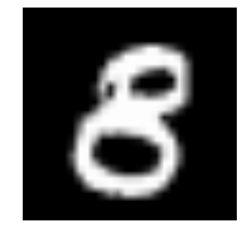
print "Prediction is: ", pred[test_index]

pylab.imshow(img, cmap='gray')
pylab.axis('off')
pylab.show()
Prediction is: 8
- We see that our model performance is pretty good! Now let’s create a submission
sample_submission.filename = test.filename; sample_submission.label = pred
sample_submission.to_csv(os.path.join(sub_dir, 'sub04.csv'), index=False)
And we’re done! We just created our own trained neural network!
Getting to know Transfer Learning and Fine Tuning
As we have seen before, training a neural network from scratch is a pain. It can require extensive training times as the number of parameters increase. But now with techniques like transfer learning, you can essentially cut short a lot of this training time.
But what is Transfer Learning? The technique can be interpreted by observing a teacher-student scenario. A teacher has years of experience in the particular topic he/she teaches. With all this accumulated information, the lectures that students get is a concise and brief overview of the topic. So it can be seen as a “transfer” of information from the learned to a novice.
Keeping in mind this analogy, we compare this to neural network. A neural network is trained on a data. This network gains knowledge from this data, which is compiled as “weights” of the network. These weights can be extracted and then transferred to any other neural network. Instead of training the other neural network from scratch, we “transfer” the learned features.
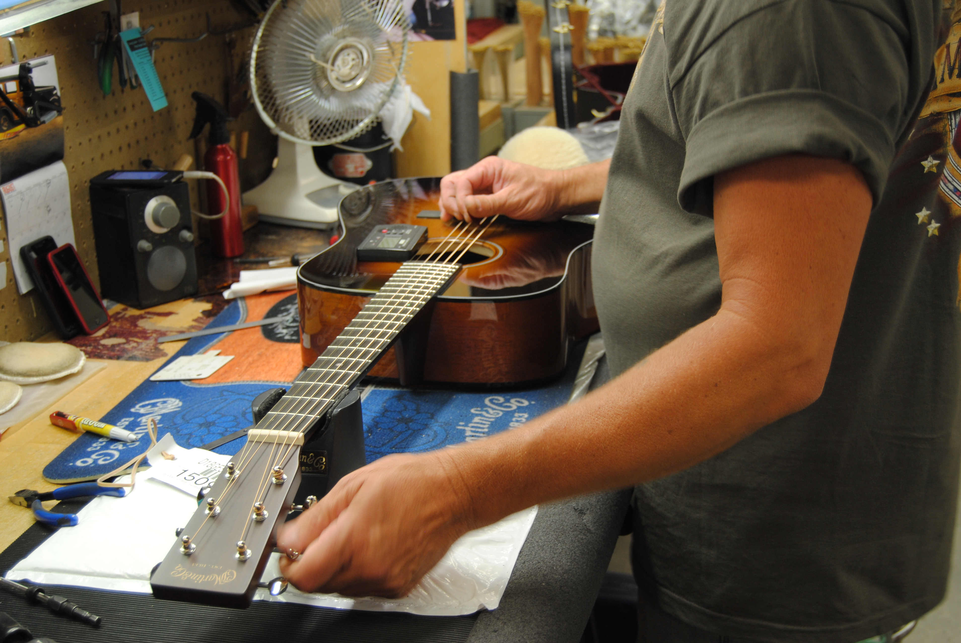
This transfer of learned features can be done across any domains. To make the models domain specific, you have to train it on the original domain. This is where fine tuning comes in. Fine tuning is retraining your model on the intended data but with decreased “learning rates”. You essentially try to change only those things which could increase your model’s overall effectiveness. Fine tuning can be considered the same as tuning strings of a guitar.
Let us try understanding the topics with an example:
Suppose you have images of dogs and you want to your model to recognize whether there’s a dog in the picture? How would you solve this problem?
We take a neural network mode, say VGG-16 (as displayed below) and train it on ImageNet data. For those who don’t know what ImageNet is, it’s a dataset comprised of tens of thousands of images with their respective labels. Training on such a big dataset is no small feat. It takes a lot of time and resources to train on such a data.
So what you would do is, download a pre-trained VGG model (which have been trained by other people) and use the weights of this model to initialize your own model. Then you retrain the model on your required problem. During retraining you can essentially “freeze” the first few layers, i.e. you can set the learning rates of these layers to 0, and continue training. You do this because you are fine-tuning your model, i.e. you adjust the parameters of a pre-trained network to better fit your data.

Case study with Keras and Theano
Now let’s jump on to a practical use case! We will be using the practice problem again, but this time we’ll be combining everything we’ve learnt uptil now and implement it. A short overview of what will do, we’ll first train a custom neural network built with Theano, extract pre-trained weights from this network and fine-tune a Keras model. Let’s go!
NOTE: Some steps we’ll see now have been explained in above code. We’re changing some parts of it to see a case study of transfer learning and fine tuning
- import modules
%pylab inline

import os
import numpy as np
import pandas as pd
from scipy.misc import imread
from sklearn.metrics import accuracy_score

import theano
import theano.tensor as T

from keras.models import Sequential
from keras.layers import Dense
- stop randomness
# To stop potential randomness
seed = 128
rng = np.random.RandomState(seed)
- set paths
root_dir = os.path.abspath('../..')
data_dir = os.path.join(root_dir, 'data', 'AV_data')
sub_dir = os.path.join(root_dir, 'sub')

# check for existence
os.path.exists(root_dir)
os.path.exists(data_dir)
- load data
train = pd.read_csv(os.path.join(data_dir, 'Train', 'train.csv'))
test = pd.read_csv(os.path.join(data_dir, 'Test.csv'))

sample_submission = pd.read_csv(os.path.join(data_dir, 'Sample_Submission.csv'))
- create train and test
temp = []
for img_name in train.filename:
    image_path = os.path.join(data_dir, 'Train', 'Images', 'train', img_name)
    img = imread(image_path, flatten=True)
    img = img.astype('float32')
    temp.append(img)

train_x = np.stack(temp)

temp = []
for img_name in test.filename:
    image_path = os.path.join(data_dir, 'Train', 'Images', 'test', img_name)
    img = imread(image_path, flatten=True)
    img = img.astype('float32')
    temp.append(img)

test_x = np.stack(temp)
- create validation
split_size = int(train_x.shape[0]*0.7)

train_x, val_x = train_x[:split_size], train_x[split_size:]
train_y, val_y = train.label.values[:split_size], train.label.values[split_size:]
train_x = train_x.reshape(-1, 784)
val_x = val_x.reshape(-1, 784)
test_x = test_x.reshape(-1, 784)
- create helper functions
def dense_to_one_hot(labels_dense, num_classes=10):
    """Convert class labels from scalars to one-hot vectors"""
    num_labels = labels_dense.shape[0]
    index_offset = numpy.arange(num_labels) * num_classes
    labels_one_hot = numpy.zeros((num_labels, num_classes))
    labels_one_hot.flat[index_offset + labels_dense.ravel()] = 1

    return labels_one_hot

def preproc(unclean_batch_x):
    """
    Convert values to range 0-1
    """
    temp_batch = unclean_batch_x / unclean_batch_x.max()

    return temp_batch

def batch_creator(batch_size, dataset_x, dataset_y):
    """
    Create batch with random samples
    """
    batch_mask = rng.choice(dataset_x.shape[0], batch_size)

    batch_x = dataset_x[batch_mask]
    batch_y = dataset_y[batch_mask]

    batch_x = preproc(batch_x)
    batch_y = dense_to_one_hot(batch_y)

    return batch_x, batch_y

def to_theano_float(arr):
    """Convert numpy array to theano tensors"""
    return np.asarray(arr, dtype=theano.config.floatX)
- set variables
# number of neurons in each layer
input_num_units = 784
hidden_num_units = 50
output_num_units = 10

# initialize theano tensors
X = T.fmatrix()
y = T.fmatrix()

# set remaining parameters
epochs = 5
batch_size = 128
- set weights and biases
weights_hidden = theano.shared(to_theano_float(rng.randn(*(input_num_units, hidden_num_units)) * 0.01))
weights_output = theano.shared(to_theano_float(rng.randn(*(hidden_num_units, output_num_units)) * 0.01))

bias_hidden = theano.shared(to_theano_float(rng.randn(hidden_num_units) * 0.01))
bias_output = theano.shared(to_theano_float(rng.randn(output_num_units) * 0.01))
- create architecture
hidden = T.nnet.relu(T.dot(X, weights_hidden) + bias_hidden)
output = T.nnet.softmax(T.dot(hidden, weights_output) + bias_output)
one_hot_to_dense = T.argmax(output, axis=1)
- set cost
cost = T.mean(T.nnet.categorical_crossentropy(output, y))
- For our case study, we’ll be changing this part. We first define our first gradient descent function
params = [weights_hidden, weights_output, bias_hidden, bias_output]

def sgd1(cost, params, lr=0.1):
    grads = T.grad(cost=cost, wrt=params)
    updates = []

    for p, g in zip(params, grads):
        updates.append([p, p - g * lr])

    return updates

updates1 = sgd1(cost, params)
- We then define our second gradient descent function
def sgd2(cost, params, lr=0.001):
    grads = T.grad(cost=cost, wrt=params)
    updates = []

    for p, g in zip(params, grads):
        updates.append([p, p - g * lr])

    return updates

updates2 = sgd2(cost, params)
- Now we compile our Theano functions
train1 = theano.function(inputs=[X, y], outputs=cost, updates=updates1, allow_input_downcast=True)
train2 = theano.function(inputs=[X, y], outputs=cost, updates=updates2, allow_input_downcast=True)
predict = theano.function(inputs=[X], outputs=one_hot_to_dense, allow_input_downcast=True)
- Let’s start training!
print 'Training with first optimizer\n'

for epoch in range(epochs):
    avg_cost = 0
    total_batch = int(train_x.shape[0]/batch_size)
    for i in range(total_batch):
            batch_x, batch_y = batch_creator(batch_size, train_x, train_y)
            c = train1(batch_x, batch_y)

            avg_cost += c / total_batch

    print 'Training accuracy:', np.mean(train_y == predict(train_x)), 'Validation accuracy:', np.mean(val_y == predict(val_x))

print '\nTraining with second optimizer\n'

for epoch in range(epochs):
    avg_cost = 0
    total_batch = int(train_x.shape[0]/batch_size)
    for i in range(total_batch):
            batch_x, batch_y = batch_creator(batch_size, train_x, train_y)
            c = train2(batch_x, batch_y)

            avg_cost += c / total_batch

    print 'Training accuracy:', np.mean(train_y == predict(train_x)), 'Validation accuracy:', np.mean(val_y == predict(val_x))
- Let’s extract weights and biases from our trained model
w_h = weights_hidden.get_value()
w_o = weights_output.get_value()

b_h = bias_hidden.get_value()
b_o = bias_output.get_value()
- Let’s create our Keras model
model = Sequential([
    Dense(output_dim=hidden_num_units, input_dim=input_num_units, activation='relu'),

    Dense(output_dim=output_num_units, activation='softmax'),
])
- Now we transfer weights from our trained model to the Keras model
model.layers[0].set_weights([w_h, b_h])

model.layers[1].set_weights([w_o, b_o])
- Let’s fine tune our model. First will free the first layer of our network.
model.layers[0].trainable = False
- Compile Keras model
model.compile(loss='categorical_crossentropy', optimizer='adam', metrics=['accuracy'], )
- Retrain model on our data
model.fit(train_x, dense_to_one_hot(train_y), nb_epoch=epochs, batch_size=batch_size, validation_data=(val_x, dense_to_one_hot(val_y)))
- Get predictions and visualize
pred = model.predict_classes(test_x)
img_name = rng.choice(test.filename)
filepath = os.path.join(data_dir, 'Train', 'Images', 'test', img_name)

img = imread(filepath, flatten=True)

test_index = int(img_name.split('.')[0]) - 49000

print "Prediction is: ", pred[test_index]

pylab.imshow(img, cmap='gray')
pylab.axis('off')
pylab.show()
Prediction is: 8
- Let’s create our submission
sample_submission.filename = test.filename; sample_submission.label = pred
sample_submission.to_csv(os.path.join(sub_dir, 'sub05.csv'), index=False)
Where to go from here
Techniques like Transfer Learning and Fine Tuning are a great way to increase the efficiency of neural networks both in terms of time and memory resources. As you saw in the case study, it’s pretty easy to implement ideas when you have an understanding of it. Tools like Theano and Keras give us the ability to go beyond what is already done, to innovate and build something useful. In reality, it is you who gets superpowers when you use them!
There are many things still unexplored in Deep Learning / Neural Networks, each and every day, there are papers being published and projects being done to push the boundaries. Therefore knowing the tools and how to leverage them is an absolute must to everyone who wants to make a dent in this field.
Additional Resources
End Notes
I hope you found this article helpful. Now, it’s time for you to practice and read as much as you can.Good Luck!
What’s your Keras vs Theano story, and which superpower do you prefer? Tell me about it in the comments below and let’s discuss further. And to gain expertise in working in neural network don’t forget to try out our deep learning practice problem – Identify the Digits.


HI Good One Can you please also try the same approach for any one of the classical classification problems . Most of the times i can find Keras for image /Digit recognition problems
Hi venugopal. Point taken. I will try what you suggested in the future . In the meantime, you can refer a similar article on AV which is an implementation of classical ML problem with neural networks ( https://www.analyticsvidhya.com/blog/2016/10/investigation-on-handling-structured-imbalanced-datasets-with-deep-learning/ )
how to save the feature vectors of a pretrained net like alexnet or vgg ie the layer before fully connected ones
Hi I like it. I need to do fine tuning for SSD architectures. I plan to use VGG16 pretrained on pascal voc datasets ( 21 classes) and I want to finetune for a single class( person) Questions: does it mean the dataset to fine tune for a single class should contain only person in different orientation ? if yes which dataset is best for this? what if I donate for the blog up to $ 100 and you intern teach me some thing in ssd fine tuning?