Introduction
One of the biggest challenge beginners in machine learning face is which algorithms to learn and focus on. In case of R, the problem gets accentuated by the fact that various algorithms would have different syntax, different parameters to tune and different requirements on the data format. This could be too much for a beginner.
So, then how do you transform from a beginner to a data scientist building hundreds of models and stacking them together? There certainly isn’t any shortcut but what I’ll tell you today will make you capable of applying hundreds of machine learning models without having to:
- remember the different package names for each algorithm.
- syntax of applying each algorithm.
- parameters to tune for each algorithm.
All this has been made possible by the years of effort that have gone behind CARET ( Classification And Regression Training) which is possibly the biggest project in R. This package alone is all you need to know for solve almost any supervised machine learning problem. It provides a uniform interface to several machine learning algorithms and standardizes various other tasks such as Data splitting, Pre-processing, Feature selection, Variable importance estimation, etc.
To get an in-depth overview of various functionalities provided by Caret, you can refer to this article.
Today, we’ll work on the Loan Prediction problem-III to show you the power of Caret package.
P.S. While caret definitely simplifies the job to a degree, it can not take away the hard work and practice you need to put in to become a master at machine learning.
Table of Contents
- Getting started
- Pre-processing using Caret
- Splitting the data using Caret
- Feature selection using Caret
- Training models using Caret
- Parameter tuning using Caret
- Variable importance estimation using Caret
- Making predictions using Caret
1. Getting started
To put in simple words, Caret is essentially a wrapper for 200+ machine learning algorithms. Additionally, it provides several features which makes it a one stop solution for all the modeling needs for supervised machine learning problems.
Caret tries not to load all the packages it depends upon at the start. Instead, it loads them only when the packages are needed. But it does assume that you already have all the algorithms installed on your system.
To install Caret on your system, use the following command. Heads up: It might take some time:
> install.packages("caret", dependencies = c("Depends", "Suggests"))Now, let’s get started using caret package on Loan Prediction 3 problem:
#Loading caret packagelibrary("caret")#Loading training datatrain<-read.csv("train_u6lujuX_CVtuZ9i.csv",stringsAsFactors = T)#Looking at the structure of caret package.str(train)#'data.frame': 614 obs. of 13 variables:#$ Loan_ID : Factor w/ 614 levels "LP001002","LP001003",..: 1 2 3 4 5 6 7 8 9 #10 ..#$ Gender : Factor w/ 3 levels "","Female","Male": 3 3 3 3 3 3 3 3 3 3 ...#$ Married : Factor w/ 3 levels "","No","Yes": 2 3 3 3 2 3 3 3 3 3 ...#$ Dependents : Factor w/ 5 levels "","0","1","2",..: 2 3 2 2 2 4 2 5 4 3 ...#$ Education : Factor w/ 2 levels "Graduate","Not Graduate": 1 1 1 2 1 1 2 1 1 #1 ...#$ Self_Employed : Factor w/ 3 levels "","No","Yes": 2 2 3 2 2 3 2 2 2 2 ...#$ ApplicantIncome : int 5849 4583 3000 2583 6000 5417 2333 3036 4006 12841 #...#$ CoapplicantIncome: num 0 1508 0 2358 0 ...#$ LoanAmount : int NA 128 66 120 141 267 95 158 168 349 ...#$ Loan_Amount_Term : int 360 360 360 360 360 360 360 360 360 360 ...#$ Credit_History : int 1 1 1 1 1 1 1 0 1 1 ...#$ Property_Area : Factor w/ 3 levels "Rural","Semiurban",..: 3 1 3 3 3 3 3 2 3 2 #...#$ Loan_Status : Factor w/ 2 levels "N","Y": 2 1 2 2 2 2 2 1 2 1 ...
In this problem, we have to predict the Loan Status of a person based on his/ her profile.
2. Pre-processing using Caret
We need to pre-process our data before we can use it for modeling. Let’s check if the data has any missing values:
sum(is.na(train))#[1] 86
Next, let us use Caret to impute these missing values using KNN algorithm. We will predict these missing values based on other attributes for that row. Also, we’ll scale and center the numerical data by using the convenient preprocess() in Caret.
#Imputing missing values using KNN.Also centering and scaling numerical columnspreProcValues <- preProcess(train, method = c("knnImpute","center","scale"))library('RANN')train_processed <- predict(preProcValues, train)sum(is.na(train_processed))#[1] 0
It is also very easy to use one hot encoding in Caret to create dummy variables for each level of a categorical variable. But first, we’ll convert the dependent variable to numerical.
#Converting outcome variable to numerictrain_processed$Loan_Status<-ifelse(train_processed$Loan_Status=='N',0,1)id<-train_processed$Loan_IDtrain_processed$Loan_ID<-NULL#Checking the structure of processed train filestr(train_processed)#'data.frame': 614 obs. of 12 variables:#$ Gender : Factor w/ 3 levels "","Female","Male": 3 3 3 3 3 3 3 3 3 3 ...#$ Married : Factor w/ 3 levels "","No","Yes": 2 3 3 3 2 3 3 3 3 3 ...#$ Dependents : Factor w/ 5 levels "","0","1","2",..: 2 3 2 2 2 4 2 5 4 3 ...#$ Education : Factor w/ 2 levels "Graduate","Not Graduate": 1 1 1 2 1 1 2 1 1 #1 ...#$ Self_Employed : Factor w/ 3 levels "","No","Yes": 2 2 3 2 2 3 2 2 2 2 ...#$ ApplicantIncome : num 0.0729 -0.1343 -0.3934 -0.4617 0.0976 ...#$ CoapplicantIncome: num -0.554 -0.0387 -0.554 0.2518 -0.554 ...#$ LoanAmount : num 0.0162 -0.2151 -0.9395 -0.3086 -0.0632 ...#$ Loan_Amount_Term : num 0.276 0.276 0.276 0.276 0.276 ...#$ Credit_History : num 0.432 0.432 0.432 0.432 0.432 ...#$ Property_Area : Factor w/ 3 levels "Rural","Semiurban",..: 3 1 3 3 3 3 3 2 3 2 #...#$ Loan_Status : num 1 0 1 1 1 1 1 0 1 0 ...
Now, creating dummy variables using one hot encoding:
#Converting every categorical variable to numerical using dummy variablesdmy <- dummyVars(" ~ .", data = train_processed,fullRank = T)train_transformed <- data.frame(predict(dmy, newdata = train_processed))#Checking the structure of transformed train filestr(train_transformed)#'data.frame': 614 obs. of 19 variables:#$ Gender.Female : num 0 0 0 0 0 0 0 0 0 0 ...#$ Gender.Male : num 1 1 1 1 1 1 1 1 1 1 ...#$ Married.No : num 1 0 0 0 1 0 0 0 0 0 ...#$ Married.Yes : num 0 1 1 1 0 1 1 1 1 1 ...#$ Dependents.0 : num 1 0 1 1 1 0 1 0 0 0 ...#$ Dependents.1 : num 0 1 0 0 0 0 0 0 0 1 ...#$ Dependents.2 : num 0 0 0 0 0 1 0 0 1 0 ...#$ Dependents.3. : num 0 0 0 0 0 0 0 1 0 0 ...#$ Education.Not.Graduate : num 0 0 0 1 0 0 1 0 0 0 ...#$ Self_Employed.No : num 1 1 0 1 1 0 1 1 1 1 ...#$ Self_Employed.Yes : num 0 0 1 0 0 1 0 0 0 0 ...#$ ApplicantIncome : num 0.0729 -0.1343 -0.3934 -0.4617 0.0976 ...#$ CoapplicantIncome : num -0.554 -0.0387 -0.554 0.2518 -0.554 ...#$ LoanAmount : num 0.0162 -0.2151 -0.9395 -0.3086 -0.0632 ...#$ Loan_Amount_Term : num 0.276 0.276 0.276 0.276 0.276 ...#$ Credit_History : num 0.432 0.432 0.432 0.432 0.432 ...#$ Property_Area.Semiurban: num 0 0 0 0 0 0 0 1 0 1 ...#$ Property_Area.Urban : num 1 0 1 1 1 1 1 0 1 0 ...#$ Loan_Status : num 1 0 1 1 1 1 1 0 1 0 ...#Converting the dependent variable back to categoricaltrain_transformed$Loan_Status<-as.factor(train_transformed$Loan_Status)
Here, “fullrank=T” will create only (n-1) columns for a categorical column with n different levels. This works well particularly for the representing categorical predictors like gender, married, etc. where we only have two levels: Male/Female, Yes/No, etc. because 0 can be used to represent one class while 1 represents the other class in same column.
3. Splitting data using caret
We’ll be creating a cross-validation set from the training set to evaluate our model against. It is important to rely more on the cross-validation set for the actual evaluation of your model otherwise you might end up overfitting the public leaderboard.
We’ll use createDataPartition() to split our training data into two sets : 75% and 25%. Since, our outcome variable is categorical in nature, this function will make sure that the distribution of outcome variable classes will be similar in both the sets.
#Spliting training set into two parts based on outcome: 75% and 25%index <- createDataPartition(train_transformed$Loan_Status, p=0.75, list=FALSE)trainSet <- train_transformed[ index,]testSet <- train_transformed[-index,]#Checking the structure of trainSetstr(trainSet)#'data.frame': 461 obs. of 19 variables:#$ Gender.Female : num 0 0 0 0 0 0 0 0 0 0 ...#$ Gender.Male : num 1 1 1 1 1 1 1 1 1 1 ...#$ Married.No : num 1 0 0 0 1 0 0 0 0 0 ...#$ Married.Yes : num 0 1 1 1 0 1 1 1 1 1 ...#$ Dependents.0 : num 1 0 1 1 1 0 1 0 0 0 ...#$ Dependents.1 : num 0 1 0 0 0 0 0 0 1 0 ...#$ Dependents.2 : num 0 0 0 0 0 1 0 0 0 1 ...#$ Dependents.3. : num 0 0 0 0 0 0 0 1 0 0 ...#$ Education.Not.Graduate : num 0 0 0 1 0 0 1 0 0 0 ...#$ Self_Employed.No : num 1 1 0 1 1 0 1 1 1 1 ...#$ Self_Employed.Yes : num 0 0 1 0 0 1 0 0 0 0 ...#$ ApplicantIncome : num 0.0729 -0.1343 -0.3934 -0.4617 0.0976 ...#$ CoapplicantIncome : num -0.554 -0.0387 -0.554 0.2518 -0.554 ...#$ LoanAmount : num 0.0162 -0.2151 -0.9395 -0.3086 -0.0632 ...#$ Loan_Amount_Term : num 0.276 0.276 0.276 0.276 0.276 ...#$ Credit_History : num 0.432 0.432 0.432 0.432 0.432 ...#$ Property_Area.Semiurban: num 0 0 0 0 0 0 0 1 1 0 ...#$ Property_Area.Urban : num 1 0 1 1 1 1 1 0 0 1 ...#$ Loan_Status : Factor w/ 2 levels "0","1": 2 1 2 2 2 2 2 1 1 2 ...
4. Feature selection using Caret
Feature selection is an extremely crucial part of modeling. To understand the importance of feature selection and various techniques used for feature selection, I strongly recommend that you to go through my previous article. For now, we’ll be using Recursive Feature elimination which is a wrapper method to find the best subset of features to use for modeling.
#Feature selection using rfe in caretcontrol <- rfeControl(functions = rfFuncs,method = "repeatedcv",repeats = 3,verbose = FALSE)outcomeName<-'Loan_Status'predictors<-names(trainSet)[!names(trainSet) %in% outcomeName]Loan_Pred_Profile <- rfe(trainSet[,predictors], trainSet[,outcomeName],rfeControl = control)Loan_Pred_Profile#Recursive feature selection#Outer resampling method: Cross-Validated (10 fold, repeated 3 times)#Resampling performance over subset size:# Variables Accuracy Kappa AccuracySD KappaSD Selected#4 0.7737 0.4127 0.03707 0.09962#8 0.7874 0.4317 0.03833 0.11168#16 0.7903 0.4527 0.04159 0.11526#18 0.7882 0.4431 0.03615 0.10812#The top 5 variables (out of 16):# Credit_History, LoanAmount, Loan_Amount_Term, ApplicantIncome, CoapplicantIncome#Taking only the top 5 predictorspredictors<-c("Credit_History", "LoanAmount", "Loan_Amount_Term", "ApplicantIncome", "CoapplicantIncome")
5. Training models using Caret
This is probably the part where Caret stands out from any other available package. It provides the ability for implementing 200+ machine learning algorithms using consistent syntax. To get a list of all the algorithms that Caret supports, you can use:
names(getModelInfo())#[1] "ada" "AdaBag" "AdaBoost.M1" "adaboost"#[5] "amdai" "ANFIS" "avNNet" "awnb"#[9] "awtan" "bag" "bagEarth" "bagEarthGCV"#[13] "bagFDA" "bagFDAGCV" "bam" "bartMachine"#[17] "bayesglm" "bdk" "binda" "blackboost"#[21] "blasso" "blassoAveraged" "Boruta" "bridge"#….#[205] "svmBoundrangeString" "svmExpoString" "svmLinear" "svmLinear2"#[209] "svmLinear3" "svmLinearWeights" "svmLinearWeights2" "svmPoly"#[213] "svmRadial" "svmRadialCost" "svmRadialSigma" "svmRadialWeights"#[217] "svmSpectrumString" "tan" "tanSearch" "treebag"#[221] "vbmpRadial" "vglmAdjCat" "vglmContRatio" "vglmCumulative"#[225] "widekernelpls" "WM" "wsrf" "xgbLinear"#[229] "xgbTree" "xyf"
To get more details of any model, you can refer here.
We can simply apply a large number of algorithms with similar syntax. For example, to apply, GBM, Random forest, Neural net and Logistic regression :
model_gbm<-train(trainSet[,predictors],trainSet[,outcomeName],method='gbm')model_rf<-train(trainSet[,predictors],trainSet[,outcomeName],method='rf')model_nnet<-train(trainSet[,predictors],trainSet[,outcomeName],method='nnet')model_glm<-train(trainSet[,predictors],trainSet[,outcomeName],method='glm')
You can proceed further tune the parameters in all these algorithms using the parameter tuning techniques.
6. Parameter tuning using Caret
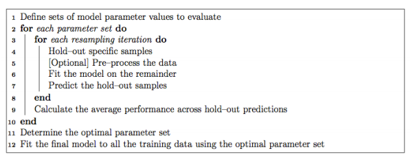
It’s extremely easy to tune parameters using Caret. Typically, parameter tuning in Caret is done as below:
It is possible to customize almost every step in the tuning process. The resampling technique used for evaluating the performance of the model using a set of parameters in Caret by default is bootstrap, but it provides alternatives for using k-fold, repeated k-fold as well as Leave-one-out cross validation (LOOCV) which can be specified using trainControl(). In this example, we’ll be using 5-Fold cross-validation repeated 5 times.
fitControl <- trainControl(method = "repeatedcv",number = 5,repeats = 5)
If the search space for parameters is not defined, Caret will use 3 random values of each tunable parameter and use the cross-validation results to find the best set of parameters for that algorithm. Otherwise, there are two more ways to tune parameters:
6.1.Using tuneGrid
To find the parameters of a model that can be tuned, you can use
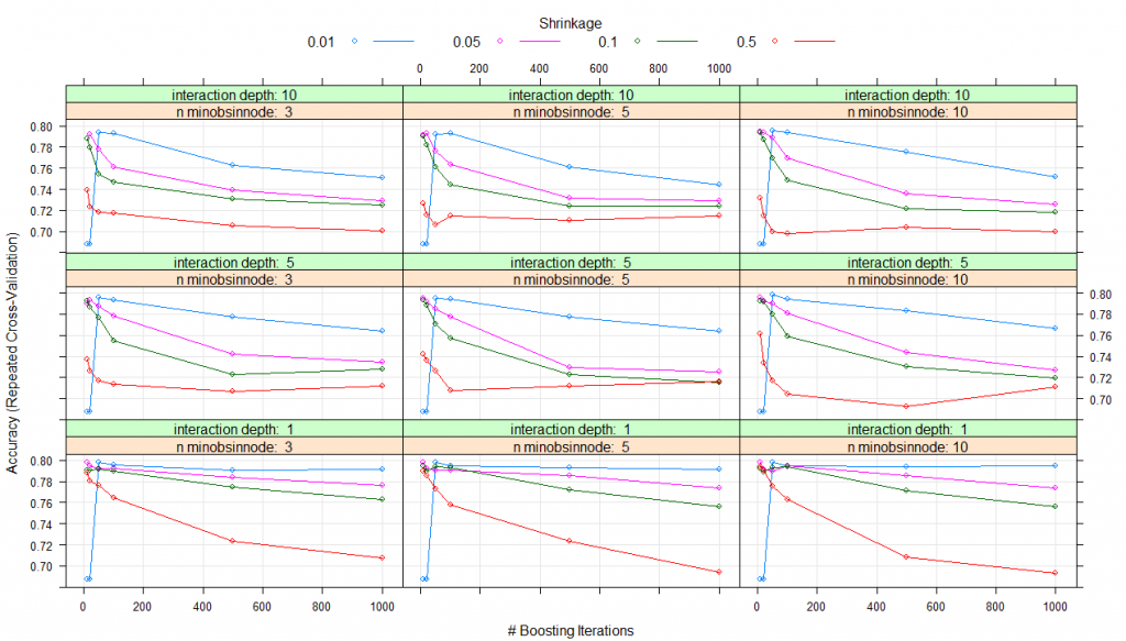
modelLookup(model='gbm')#model parameter label forReg forClass probModel#1gbmn.trees # Boosting Iterations TRUE TRUE TRUE#2gbminteraction.depth Max Tree Depth TRUE TRUE TRUE#3gbmshrinkage Shrinkage TRUE TRUE TRUE#4gbmn.minobsinnode Min. Terminal Node Size TRUE TRUE TRUE#using grid search#Creating gridgrid <- expand.grid(n.trees=c(10,20,50,100,500,1000),shrinkage=c(0.01,0.05,0.1,0.5),n.minobsinnode = c(3,5,10),interaction.depth=c(1,5,10))# training the modelmodel_gbm<-train(trainSet[,predictors],trainSet[,outcomeName],method='gbm',trControl=fitControl,tuneGrid=grid)# summarizing the modelprint(model_gbm)#Stochastic Gradient Boosting#461 samples#5 predictor#2 classes: '0', '1'#No pre-processing#Resampling: Cross-Validated (5 fold, repeated 5 times)#Summary of sample sizes: 368, 370, 369, 369, 368, 369, ...#Resampling results across tuning parameters:# shrinkage interaction.depth n.minobsinnode n.trees Accuracy Kappa#0.01 1 3 10 0.6876416 0.0000000 #0.01 1 3 20 0.6876416 0.0000000#0.01 1 3 50 0.7982345 0.4423609#0.01 1 3 100 0.7952190 0.4364383#0.01 1 3 500 0.7904882 0.4342300#0.01 1 3 1000 0.7913627 0.4421230#0.01 1 5 10 0.6876416 0.0000000#0.01 1 5 20 0.6876416 0.0000000#0.01 1 5 50 0.7982345 0.4423609#0.01 1 5 100 0.7943635 0.4351912#0.01 1 5 500 0.7930783 0.4411348#0.01 1 5 1000 0.7913720 0.4417463#0.01 1 10 10 0.6876416 0.0000000#0.01 1 10 20 0.6876416 0.0000000#0.01 1 10 50 0.7982345 0.4423609#0.01 1 10 100 0.7943635 0.4351912#0.01 1 10 500 0.7939525 0.4426503#0.01 1 10 1000 0.7948362 0.4476742#0.01 5 3 10 0.6876416 0.0000000#0.01 5 3 20 0.6876416 0.0000000#0.01 5 3 50 0.7960556 0.4349571#0.01 5 3 100 0.7934987 0.4345481#0.01 5 3 500 0.7775055 0.4147204#...#0.50 5 10 100 0.7045617 0.2834696#0.50 5 10 500 0.6924480 0.2650477#0.50 5 10 1000 0.7115234 0.3050953#0.50 10 3 10 0.7389117 0.3681917#0.50 10 3 20 0.7228519 0.3317001#0.50 10 3 50 0.7180833 0.3159445#0.50 10 3 100 0.7172417 0.3189655#0.50 10 3 500 0.7058472 0.3098146#0.50 10 3 1000 0.7001852 0.2967784#0.50 10 5 10 0.7266895 0.3378430#0.50 10 5 20 0.7154746 0.3197905#0.50 10 5 50 0.7063535 0.2984819#0.50 10 5 100 0.7151012 0.3141440#0.50 10 5 500 0.7108516 0.3146822#0.50 10 5 1000 0.7147320 0.3225373#0.50 10 10 10 0.7314871 0.3327504#0.50 10 10 20 0.7150814 0.3081869#0.50 10 10 50 0.6993723 0.2815981#0.50 10 10 100 0.6977416 0.2719140#0.50 10 10 500 0.7037864 0.2854748#0.50 10 10 1000 0.6995610 0.2869718
Accuracy was used to select the optimal model using the largest value.
The final values used for the model were n.trees = 10, interaction.depth = 1, shrinkage = 0.05 and n.minobsinnode = 3
plot(model_gbm)
Thus, for all the parameter combinations that you listed in expand.grid(), a model will be created and tested using cross-validation. The set of parameters with the best cross-validation performance will be used to create the final model which you get at the end.
6.2. Using tuneLength
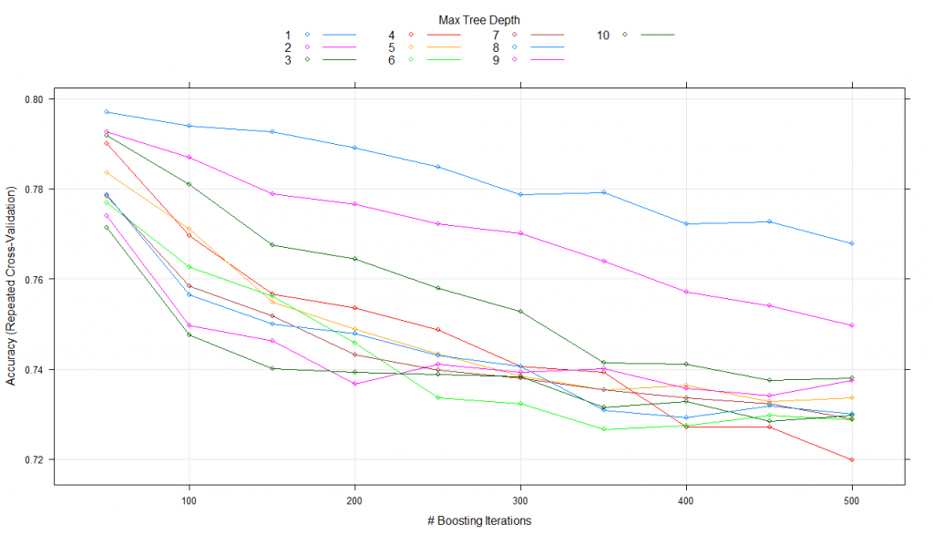
Instead, of specifying the exact values for each parameter for tuning we can simply ask it to use any number of possible values for each tuning parameter through tuneLength. Let’s try an example using tuneLength=10.
#using tune lengthmodel_gbm<-train(trainSet[,predictors],trainSet[,outcomeName],method='gbm',trControl=fitControl,tuneLength=10)print(model_gbm)#Stochastic Gradient Boosting#461 samples#5 predictor#2 classes: '0', '1'#No pre-processing#Resampling: Cross-Validated (5 fold, repeated 5 times)#Summary of sample sizes: 368, 369, 369, 370, 368, 369, ...#Resampling results across tuning parameters:# interaction.depth n.trees Accuracy Kappa#1 50 0.7978084 0.4541008#1 100 0.7978177 0.4566764#1 150 0.7934792 0.4472347#1 200 0.7904310 0.4424091#1 250 0.7869714 0.4342797#1 300 0.7830488 0.4262414...#10 100 0.7575230 0.3860319#10 150 0.7479757 0.3719707#10 200 0.7397290 0.3566972#10 250 0.7397285 0.3561990#10 300 0.7362552 0.3513413#10 350 0.7340812 0.3453415#10 400 0.7336416 0.3453117#10 450 0.7306027 0.3415153#10 500 0.7253854 0.3295929
Tuning parameter ‘shrinkage’ was held constant at a value of 0.1
Tuning parameter ‘n.minobsinnode’ was held constant at a value of 10
Accuracy was used to select the optimal model using the largest value.
The final values used for the model were n.trees = 50, interaction.depth = 2, shrinkage = 0.1 and n.minobsinnode = 10.
plot(model_gbm)
Here, it keeps the shrinkage and n.minobsinnode parameters constant while alters n.trees and interaction.depth over 10 values and uses the best combination to train the final model with.
7. Variable importance estimation using caret
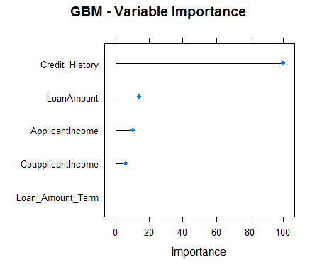
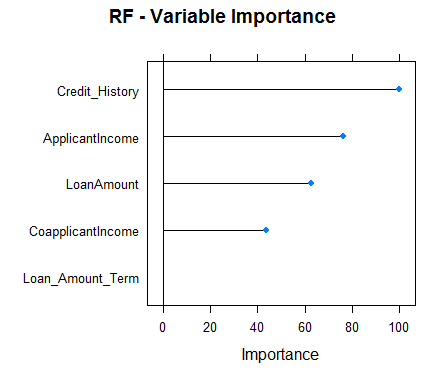
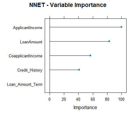
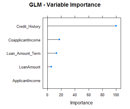
Caret also makes the variable importance estimates accessible with the use of varImp() for any model. Let’s have a look at the variable importance for all the four models that we created:
#Checking variable importance for GBM#Variable ImportancevarImp(object=model_gbm)#gbm variable importance#Overall#Credit_History 100.000#LoanAmount 16.633#ApplicantIncome 7.104#CoapplicantIncome 6.773#Loan_Amount_Term 0.000#Plotting Varianle importance for GBMplot(varImp(object=model_gbm),main="GBM - Variable Importance")
#Checking variable importance for RFvarImp(object=model_rf)#rf variable importance#Overall#Credit_History 100.00#ApplicantIncome 73.46#LoanAmount 60.59#CoapplicantIncome 40.43#Loan_Amount_Term 0.00#Plotting Varianle importance for Random Forestplot(varImp(object=model_rf),main="RF - Variable Importance")
#Checking variable importance for NNETvarImp(object=model_nnet)#nnet variable importance#Overall#ApplicantIncome 100.00#LoanAmount 82.87#CoapplicantIncome 56.92#Credit_History 41.11#Loan_Amount_Term 0.00#Plotting Variable importance for Neural Networkplot(varImp(object=model_nnet),main="NNET - Variable Importance")
#Checking variable importance for GLMvarImp(object=model_glm)#glm variable importance#Overall#Credit_History 100.000#CoapplicantIncome 17.218#Loan_Amount_Term 12.988#LoanAmount 5.632#ApplicantIncome 0.000#Plotting Variable importance for GLMplot(varImp(object=model_glm),main="GLM - Variable Importance")
Clearly, the variable importance estimates of different models differs and thus might be used to get a more holistic view of importance of each predictor. Two main uses of variable importance from various models are:
- Predictors that are important for the majority of models represents genuinely important predictors.
- Foe ensembling, we should use predictions from models that have significantly different variable importance as their predictions are also expected to be different. Although, one thing that must be make sure is that all of them are sufficiently accurate.
8. Predictions using Caret
For predicting the dependent variable for the testing set, Caret offers predict.train(). You need to specify the model name, testing data. For classification problems, Caret also offers another feature named type which can be set to either “prob” or “raw”. For type=”raw”, the predictions will just be the outcome classes for the testing data while for type=”prob”, it will give probabilities for the occurrence of each observation in various classes of the outcome variable.
Let’s take a look at the predictions from our GBM model:
#Predictionspredictions<-predict.train(object=model_gbm,testSet[,predictors],type="raw")table(predictions)#predictions#0 1#28 125
Caret also provides a confusionMatrix function which will give the confusion matrix along with various other metrics for your predictions. Here is the performance analysis of our GBM model:
confusionMatrix(predictions,testSet[,outcomeName])#Confusion Matrix and Statistics#Reference#Prediction 0 1#0 25 3#1 23 102#Accuracy : 0.8301#95% CI : (0.761, 0.8859)#No Information Rate : 0.6863#P-Value [Acc > NIR] : 4.049e-05#Kappa : 0.555#Mcnemar's Test P-Value : 0.0001944#Sensitivity : 0.5208#Specificity : 0.9714#Pos Pred Value : 0.8929#Neg Pred Value : 0.8160#Prevalence : 0.3137#Detection Rate : 0.1634#Detection Prevalence : 0.1830#Balanced Accuracy : 0.7461#'Positive' Class : 0
Additional Resources
- Caret Package Homepage
- Caret Package on CRAN
- Caret Package Manual (PDF, all the functions)
- A Short Introduction to the caret Package (PDF)
- Open source project on GitHub (source code)
- Here is a webinar by creater of Caret package himself
End Notes
Caret is one of the most powerful and useful packages ever made in R. It alone has the capability to fulfill all the needs for predictive modeling from preprocessing to interpretation. Additionally, its syntax is also very easy to use. If you use R, I’ll encourage you to use Caret.
Caret is a very comprehensive package and instead of covering all the functionalities that it offers, I thought it’ll be a better idea to show an end-to-end implementation of Caret on a real hackathon J dataset. I have tried to cover as many functions in Caret as I could, but Caret has a lot more to offer. For going in depth, you might find the resources mentioned above very useful. Several of these resources have been written by Max Kuhn (the creator of caret package) himself.


Hello @Saurav Kaushik , I really appreciate you for sharing such a nice article on CART. This really help a lot !
Hey Kishore. Glad you liked it. Happy to help!
where can I download the data used in this article? thank you. zhanyou
Hey Zhanyou. The dataset used is from a practice problem and can be accessed at: https://datahack.analyticsvidhya.com/contest/practice-problem-loan-prediction-iii/
Hi Saurav, how are you, nice article!. Saurav, where can I download the data file? train_u6lujuX_CVtuZ9i.csv Thanks, Miguel
Hey Miguel. Thanks. You can get the data from the following practice problem: https://datahack.analyticsvidhya.com/contest/practice-problem-loan-prediction-iii/