Overview
- Generative models and GANs are at the core of recent progress in computer vision applications
- This article will introduce you to the world of GANs and its different components
- Some exciting-real world GANs use cases await – let’s dive in!
Introduction
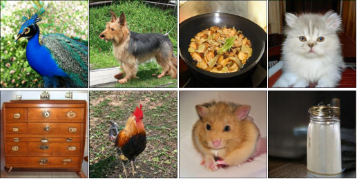
Can you pick out what’s odd in the below collection of images:
How about this one?
All of the objects and animals in these images have been generated by a computer vision model called Generative Adversarial Networks (GANs)! This is one of the most popular branches of deep learning right now. It certainly helps that they spark our hidden creative streak!
GANs are definitely one of my favorite topics in the deep learning space. I love the variety of different applications we can make using these models – from generating new faces to creating paintings (and filling in missing parts in old paintings)!
This article is all about introducing you to the world of generative networks and GANs. We will also look at the various applications of these generative networks and deep dive into the components that make them work.
Get ready for the data event of the year! Join us at the DataHack Summit 2023, happening from Aug 2-5 at the prestigious NIMHANS Convention Center in Bengaluru. Why should you be there? Well, this is your chance to dive into mind-blowing workshops, gain insights from industry experts, and connect with like-minded data enthusiasts. Stay ahead of the curve, learn the latest trends, and unlock endless possibilities in the world of data science and AI. Don’t miss out on this incredible opportunity! Mark your calendars and secure your spot at the DataHack Summit 2023. Click here for more details!
Table of Contents
- What are Generative Models?
- Applications of Generative Models
- Types of Generative Models
- Explicit Density
- Implicit Density
- Understanding Explicit Density Models
- Introduction to Generative Adversarial Networks (GANs)
- The Step-by-Step Training Process of GANs
What are Generative Models?
Let’s understand the idea behind generative models first before we look extensively at its applications. This will help you visualize the different use cases and also later relate to them when we talk about GANs.
There are broadly two major types of problems we work on in Machine Learning or Deep Learning – Supervised Learning and Unsupervised Learning.
In supervised learning problems, we have the independent variables (x) and the target label (y). The aim is to learn a mapping function to map x and y:
![]()
Examples of supervised learning include classification, regression, object detection, image segmentation, etc.
Unsupervised learning problems, on the other hand, only have the independent variables (x) and no target label. The aim here is to learn some underlying patterns from the data. Examples of unsupervised learning include clustering, dimensionality reduction, etc.
So where do generative models fit in?
When we’re provided the training data, generative models generate new samples from the training set distribution. Let’s say we have a training set having the distribution pdata(x). We want to generate samples such that the distribution of generated samples pmodel(x) is similar to pdata(x). Let me simplify this a bit more.
Using generative models, we first learn the distribution of the training set and then generate some new observations or data points using the learned distribution with some variations.
Now, there are multiple ways to learn this mapping between the model distribution and true distribution of the data which we will discuss in the later sections. Before that, let me show you a few awesome generative applications that might excite you about generative models.
Applications of Generative Models
Why do we need generative models in the first place? Even I had this question initially. But the more applications I came across, the more I was convinced by the power of generative models.
So, let me explain some of the use cases of generative models in this section to answer this question.
Generating Data
Have you ever tried building a deep learning model from scratch? One of the most common challenges most of us face is the lack of training data. Even if you have a lot of data, I’m sure you wouldn’t mind getting more! Who doesn’t love more data?
There are certain industries where we need more data to train deeper and deeper models. The Healthcare industry is a good example. Generative models can play a vital role here as they can be used to generate new data. These generated images can be used to increase your dataset size. Here is a cool example of generative models being used to generate examples of bedrooms.
We can also use generative models to generate faces. This paper demonstrates the generation of realistic photographs of human faces. There are multiple such use cases where we can use generative models to generate data – cartoon characters, images of celebrities, etc.
Image to Image Translation
I am especially fond of this generative model application. You can do some interesting stuff like translating satellite photographs to Google Maps, converting day photos into night one, black and white pictures to color photos, changing the season (let’s say summer to winters):
These are all image-to-image translation tasks. This paper illustrates the approach of many image-to-image translation tasks.
Face Aging and De-Aging
Face aging and de-aging is a process of rendering a face image with natural aging and de-aging on the individual faces:
This can be used to recognize cross-age faces, and for entertainment purposes as well. Feel free to refer to this paper if you wish to get more details on it.
There are many more applications of generative models, like 3D object generation, attention prediction, text-to-image translation, etc. Excited? Let’s start with understanding different types of generative models.
Types of Generative Models
There are two types of generative models:
- Explicit density models
- Implicit density models
Let’s first look at the below table to understand the difference between these two:
| Explicit Density | Implicit Density |
| Assumes some prior distribution about the data | Defines a stochastic procedure that directly generates data |
| Example: Maximum Likelihood | Example: Generative Adversarial Networks (GANs) |
Explicit density models define an explicit density function pmodel(x;Ө), whereas implicit density models define a stochastic procedure that can directly generate data.
Here is a visual by Ian Goodfellow that demonstrates different types of generative models:
Let’s understand these generative models in more detail.
Understanding Explicit Density Models
We know that an explicit density model defines an explicit density function. Then, it tries to maximize the likelihood of that function on the training data. Depending on whether these explicit density models are tractable or not, we can further divide them into subparts:
- Tractable density
- Approximate density
Tractable means that we can define a parametric function that is able to capture the distribution efficiently. But many of the distributions, like the distribution of images or the distribution of speech waves, are complex and it is very difficult to design a parametric function to capture them. Such models that do not have a parametric function to capture the distribution fall under approximate density models.
To define the density function, we decompose the likelihood of an image (x) into a product of 1-d distributions using the chain rule:
p(x) here represents the likelihood of image x and the right side represents the probability of the ith pixel value given all previous pixels. After defining this function, we maximize the likelihood of training data. This is how tractable explicit density models work.
Pixel RNN and Pixel CNN are the most commonly used tractable density models. Let’s discuss them in a bit more detail below.
Pixel RNN
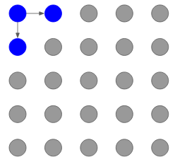
Pixel RNN is a deep neural network that generates image pixels sequentially. It starts generating the pixels from the corner and then generates the two consecutive pixels. Let me illustrate this with an example.
Let’s say we have to generate a 5×5 image. It will have 25 pixel values as shown below:
The model will start with generating the pixel from the corner:
Then, it will generate the corresponding two pixels using this corner pixel:
And this process continues till the last pixel is generated:
The generation of a pixel is dependent on all the previous pixel values and this dependency is modeled using a Recurrent Neural Network (RNN) or a Long Short Term Memory (LSTM).
This is a brief overview of how Pixel RNN works. You can check out the official Pixel RNN paper to read more about it in depth.
The drawback of using Pixel RNN is that since the generation is sequential, it is slow. This is why the Pixel CNN was introduced.
Pixel CNN
The idea of Pixel CNN is quite similar to Pixel RNN. But, instead of modeling the dependencies of previous pixels using an RNN, we use CNN over a context region. We start from the corner, just like we did in Pixel RNN, and then generate the two consecutive pixels.
To generate a pixel, let’s say xi, the model can only use the previously generated pixels, i.e. x1, x2, …, xi-1. We use a masked filter to ensure this happens:
So, the pixels which have been generated have a value of 1 and the remaining are assigned the value 0. This will take into account only the generated pixel values. Training in the case of Pixel CNN is faster as compared to the training time of Pixel RNN, but the generation of pixels is still sequential and hence the process is slow.
To summarize, both Pixel RNN and Pixel CNN can compute the likelihood p(x) explicitly which gives us a good evaluation metric to gauge our model’s performance. And we saw above that the generated samples are good. On the other hand, the generation from these models is slow as it is a sequential process.
So far, we have seen the tractable density functions. We can directly optimize the likelihood of these functions on training data. Now, we will discuss one more generative model called Variational Autoencoders (VA).
Brief Summary of how Autoencoders Work
Let’s quickly understand what autoencoders are and then we will discuss the concept of variational autoencoders and how we can use them to generate images.
Autoencoders are an unsupervised way of learning the lower-dimensional feature representations.
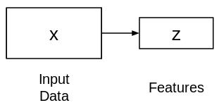
They are comprised of two connected networks – encoder and decoder. The aim of an encoder is to take an input (x) and produce a feature map (z):
The shape of this feature map (z) is usually smaller than x. Why do you think this is the case?
Since we want z to capture only the meaningful factors of variations that can describe the input data, the shape of z is usually smaller than x. Now, the question is how do we learn this feature representation (z)? How do we train this model? For that, we can add a decoder network on top of the extracted features and use L2 loss to train the model:
This is how the autoencoder network looks. This network is trained in such a way that the features (z) can be used to reconstruct the original input data (x). If the output (Ẋ) is different from the input (x), the L2 loss penalizes it and helps to reconstruct the input data.
Now, how can we generate new images from these autoencoders?
Variational Autoencoders
This is where variational autoencoders are helpful. They assume that the training data is generated from some underlying unobserved representations (z).
The main difference between a simple autoencoder and variational autoencoder is that instead of directly extracting the features from the input data, we try to model the probability distribution of the training data.
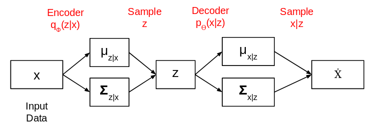
For this, instead of making the encoder output an encoding vector of size n, we output two vectors of size n – a vector of means and another vector of standard deviation.
The complete network architecture of variational autoencoders looks like this:
The mean here controls the position where the encodings of input should be centered around and the standard deviation controls how much the mean encodings can vary. The loss function that is used to train this variational autoencoder is Kullback-Leibler divergence (or the KL divergence). It measures how different two probability distributions are:
We need to minimize the KL divergence. This optimizes the parameters of the probability distribution (mean and standard deviation). Once this model is trained, we can generate new images from it. Let me show you how.
How can we generate images using Variational Autoencoders?
Once the model is trained, we remove the encoder part and get the below network:
We now pick a simple probability distribution with mean 0 and standard deviation 1 and pass it as input to the above network. It then generates an output. This is how variational autoencoders can help us generate images.
Although this method is very useful for generating images, there are a few downsides to it too. One of the major drawbacks of variational autoencoders is that the generated samples are blurrier and of low quality as compared to the samples from state-of-the-art GANs. This is an active field of research – let’s hope we see improvements soon!
So far, all the generative models we’ve seen define an explicit density function. What if we don’t want to explicitly model the density but just the ability to sample from the training set implicitly? This is where GANs come in. They have an implicit density function which helps to sample from the training set.
Introduction to Generative Adversarial Networks (GANs)
Let me illustrate an architecture first which will make understanding GANs much easier:
GANs are composed of two different networks:
- Generator Network
- Discriminator Network
Let me explain each network in detail.
Generator Network
The aim of the generator network is to generate images given some random noise as input:
This generator network is a neural network or a convolutional neural network (CNN). We pass some random noise and this network generates an image using that noise.
Discriminator Network
The job of a discriminator network is pretty simple. It has to identify whether the input is real or fake:
All the images from the training set are marked as Real (or 1) and all the generated images from the generator network are marked as Fake (or 0). Now, the task of a discriminator network is to perform binary classification. It has to classify the input as real or fake (1 or 0).
The advantage of this model is that it is completely differentiable. Since both generator and discriminator are neural networks (or convolutional neural networks), we get a completely differentiable network.
We train the model, calculate the loss function at the end of the discriminator network and backpropagate the loss into both discriminator and generator models.
This updates the parameters of both networks and subsequently improve the results. Both generator and discriminator are trained jointly in a minimax game:
Here:
- p(data) represents the distribution of data from the training set
- D(x) is the probability that x comes from the training data
- p(z) represents the input noise variable
Discriminator (D) wants to maximize the objective function such that D(x) is close to 1 and D(G(z)) is close to 0. It simply means that the discriminator should identify all the images from the training set as Real (1) and all the generated images as Fake (0).
Generator (G) wants to minimize the objective function such that D(G(z)) is 1. This means that the generator tries to generate images that are classified as Real (1) by the discriminator network.
This is how a Generative Adversarial Network (GAN) works. Let’s now discuss the step-by-step process of training GANs.
The Step-by-Step Training Process of GANs
Here’s how GANs are trained:
- First, we take a noise sample from a random distribution, feed it to the Generator (G) network, and generate some image (Fake image, label = 0):

- Then, we take fake images (label = 0) generated from the generator network and real images from the training set (label = 1) and feed these pairs to the Discriminator (D) network which classifies them:

- As you must have observed, the discriminator is a binary classifier. It calculates the loss (can be binary cross-entropy)
- We then backpropagate this loss to the discriminator and generator networks and update their weights. We can choose Adam or any other optimizer for back propagation.
This is the process of how a GAN is trained.
End Notes
GANs are an active field of research. We’re seeing regular updates almost weekly on the next GAN version. You can check out the work researchers have done here.
In my next article, I will be taking up a case study and demonstrating the implementation aspect of Generative Adversarial Networks (GANs) to generate new images. A whole lot of fun awaits us!
Connect with me in the comments section below if you have any ideas, thoughts, or suggestions on GANs!
And if you’re new to deep learning and computer vision, you should definitely check out our comprehensive course:
This is it for this article. But before you go, I’d highly recommend you check out our value-loaded workshops like ‘Mastering LLMs: Training, Fine-tuning, and Best Practices‘, ‘Exploring Generative AI with Diffusion Models‘ and ‘Solving Real World Problems Using Reinforcement Learning’ and many more at the DataHack Summit 2023 to level up your data game! Our workshops are your ticket to unlocking immense value, equipping you with practical skills and real-world knowledge that you can apply right away. Picture yourself diving into hands-on experiences, gaining the confidence to conquer any data challenge that comes your way. This is your golden opportunity to enhance your expertise, connect with industry leaders, and open doors to exciting new career opportunities. Don’t wait any longer! Secure your spot and register now for the highly anticipated DataHack Summit 2023.


Thank you for this useful article. I have a question - what is the purpose of the random noise as input to the Generator network? And once the network is trained, what do you input in place of the random noise that was input during training? Again some random noise? How does the Generator work with random input? Neural Networks generally work with some well defined data.