5 Handy Excel Tricks for Conditional Formatting Every Analyst Should Know

Overview

• Conditional formatting is a useful and powerful feature in Microsoft Excel that you should master
• We’ll discuss 5 handy conditional formatting tricks here and show you how you can use them in your analytics projects

Introduction

Let me share a quick story with you from one of my recent analytics projects. I was working in Excel with a big dataset that had a ton of numeric features (mostly sales numbers about different products). I wanted to quickly highlight a few values that any leadership team or decision-maker would instantly look at.

This kind of visualization, or analysis, is highly valued in the industry. If you can take a bunch of numbers and bring out exactly what you want to show to your audience – that is where a business analyst, data analyst, or even a data scientist stands out from the rest. And Excel is the perfect tool to extract and highlight insights using a feature called conditional formatting.

I quickly moved into the Conditional Formatting options, picked the color scales I wanted, and Excel instantly highlighted the highest and lowest sales numbers for each region and product. With just a few clicks (and an understanding of conditional formatting in Excel!), you can easily prepare and present an impactful and effective analysis to your audience.

I personally use conditional formatting a LOT as it helps me stay organized and helps me understand the data much more intuitively.

But conditional formatting can appear a bit daunting if you’re new to Excel. There are a plethora of options to choose from and picking one isn’t as straightforward. So here, I have compiled a list of 5 Excel tricks to make you a champion in conditional formatting. These tricks are beginner-friendly so even if you use Excel to record your expenses, these will definitely make you more productive.

I encourage you to check out the below resources if you’re a beginner in Excel and business analytics:

• Microsoft Excel: From Beginner to Advanced
• Microsoft Excel: Formulas and Functions (Free Course!)
• Certified Business Analytics Program (Comprehensive Multi-Course Program)

Table of Contents

1. Conditional Formatting Trick #1 – Highlight cell values greater than the average
2. Conditional Formatting Trick #2 – Highlight Sales Data with multiple formatting
3. Conditional Formatting Trick #3 – Highlight complete row if the condition is satisfied
4. Conditional Formatting Trick #4 – Highlight rows having duplicate values
5. Conditional Formatting Trick #5 – Highlight rows having multiple conditions

Conditional Formatting Trick #1 – Highlight cell values greater than the average

Let us start with an easy yet powerful Conditional Formatting trick. As the name suggests, this helps us in highlighting the cell values that satisfy a certain condition. Excel doesn’t provide a straightforward option to highlight a cell based on a condition applied to another cell so let us see how we can do this.

We will take up a problem statement where we are provided with marks of students appearing for the preliminary round of an examination. The students must achieve marks greater than the average marks of all students to proceed to the next round. Our job is to highlight the students who satisfy this condition.

We will solve this problem step-by-step so let’s get started.

Step 1: Conditional Formatting Rules Manager

To start with the analysis, open Conditional Formatting -> Manage Rules. 

Now you are in the Conditional Formatting Rules Manager. All your conditional formatting rules will be present here. Let us see how to make our first conditional formatting rule:

Step 2: Select New Rule Type

To make a new conditional formatting rule, go to New Rule. All the rule types will be present there. Since we will be making our own formula to select the column, we will choose “Use a formula to select which cells to format“:

Step 3: Enter the custom formula

Finally, we will enter our custom formula to highlight the cells in students whose values in the Preliminary round marks columns is more than the average of all the student marks:

Step 4: Choose an appropriate format

Here, I am choosing to highlight student cells in green whose marks are more than the average marks. It is up to you and you may select any other formatting style as well:

Step 5: Select the intended cells to format

Select the column to which you want to apply the formatting. In this case, it is the students column. Press the apply button and watch the magic unfold:

We have successfully completed the first problem statement!

Conditional Formatting Trick #2 – Highlight Sales Data with multiple formatting

In the previous trick, we applied a single formatting rule. Now, let us see how we can apply multiple formattings in our sheet by taking another example.

Let us take a problem statement where we have sales data for the years 2019 and 2020. This data is of a company that sells a range of products. We need to highlight the products that have increased sales with green color and the products which have decreased sales with red. Let’s begin!

Let us get started:

Select the cells you want to highlight, in this case, Products 1 – Product 7($D$4:$D$10). After this, follow steps 1 and 2 from the previous section to open the Conditional Formatting Rules Manager.

Step 3: Enter first rule

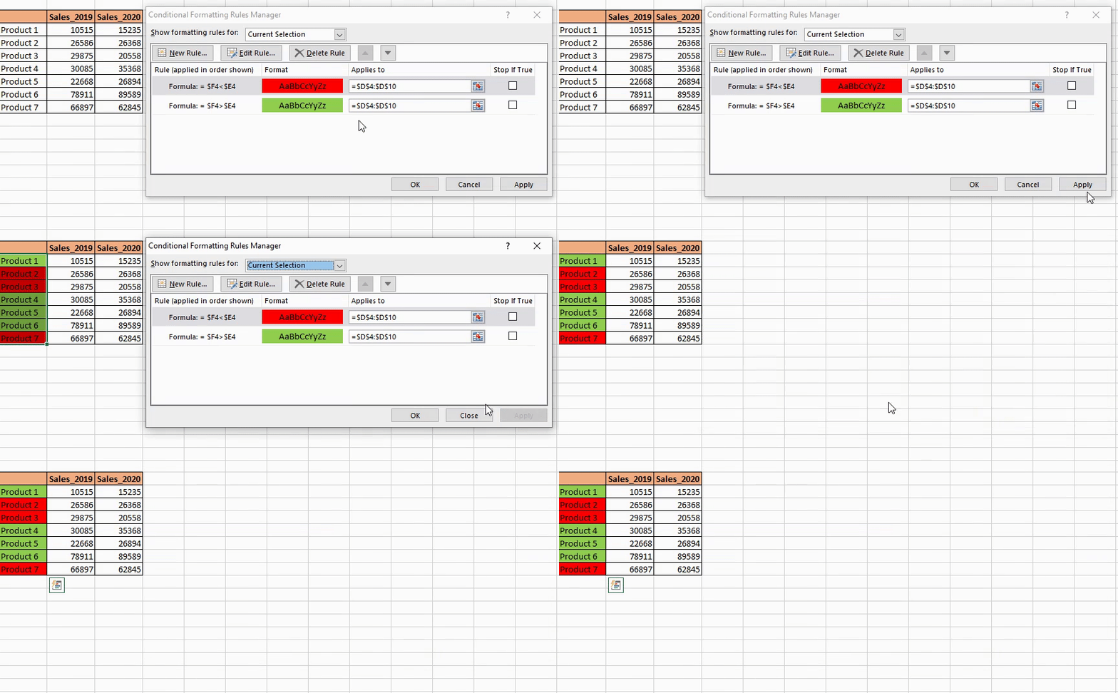
We will enter our first rule, i.e., to highlight the product cells having Sales_2020 greater than Sales_2019. We’ll be using green fill to highlight these cells:

Step 4: Enter the second rule

Now it is time to apply the second rule, i.e., to highlight the product cells having Sales_2020 less than Sales_2019. We’ll be using red fill to highlight these cells:

Step 5: Apply the format

We are ready with the two formatting rules. Make sure you have selected the correct range of intended cells. Just press Apply and voila! You have applied multiple formattings!

Conditional Formatting Trick #3 – Highlight complete row if the condition is satisfied

In real-world scenarios and analytics projects, you will come across datasheets spread across many columns and rows. In these conditions, it is desirable to format the complete row instead of just one cell.

To do this, let us take a very interesting problem statement. We are provided with the information of passengers entering the Delhi airport. We have to highlight the record of people not wearing a mask so that further action can be taken against them.

We will begin by applying Steps 1 and 2 from the first section to open the Conditional Formatting Rule Manager.

Step 3: Apply the Formula

This is the easy part. Select the formula $H5=”No” and select appropriate formatting. This is going to select all the customers who are not wearing a mask and format them as Red in this case:

Step 4: Select the range and apply

Finally, we will select the range of intended cells. Since we need to highlight the complete rows, we select all the cells and then apply the formatting:

Conditional Formatting Trick #4 – Highlight rows having duplicate values

One of the most important steps of data analysis is to detect duplicate values in your data. Excel provides a lightning-fast option to detect and visualize duplicate values in our datasets.

Let’s deep dive into our problem statement. Here, we have the order details of an e-commerce company. Our job is to highlight the customers who have made multiple transactions. Let’s see what is the fastest way to do it.

You know the drill by now -head over to the step-by-step breakdown after it.

Step 1: Select the Range

We will start off by choosing a preferred range to which we want to apply our formatting, in our case, Customer ID:

Step 2: Highlight Duplicate Values

Next, we’ll do the aforementioned highlighting of duplicate values. Go to Conditional Formatting -> Highlight cell rules ->Duplicate values:

Step 3: Select an appropriate formatting

You’ll be provided with two dropdowns. In the first dropdown, we will select “Duplicate” as we need to format only columns having duplicate values, and then we will select an appropriate highlighting format:

That’s it!

Conditional Formatting Trick #5 – Highlight rows having multiple conditions

So far, we have highlighted columns based on a single condition. Now, I want to take things up a notch. We will be applying multiple conditions and highlighting the records accordingly.

We are again going to take up an interesting problem statement. Here, we have a list of students in the final year of their graduation. The college authorities need to return the security deposits to its students but there’s a catch  – the deposit will be given only to those students who have received the approval from all the departments, i.e., Library, Sports department, and Laboratory.

We will begin by selecting the complete range of cells and repeat steps 1 and 2 from the first section.

Step 3: Apply the conditions

According to our condition, we will make a custom formula. We’ll be making use of the AND operator as we need to make sure that all the departments have given their approval to the student.

We’ll be using Green Fill as the highlighting color here:

Step 4: Apply the formatting

Let us apply the formatting and we have completed our fifth problem statement. Awesome!

End Notes

In this article, we covered five Excel tricks for conditional formatting. I hope these tricks will help you with day-to-day niche tasks and save you a lot of time.

Do you have your own conditional formatting tricks to share? Or any other Excel tricks, in general, you would want the community to know? Share them in the comments section below!

Ram Dewani

Product Growth Analyst at Analytics Vidhya. I'm always curious to deep dive into data, process it, polish it so as to create value. My interest lies in the field of marketing analytics.