Introduction to ANOVA for Statistics and Data Science (with COVID-19 Case Study using Python)

Introduction

“A fact is a simple statement that everyone believes. It’s innocent, unless found guilty. A Hypothesis is a novel suggestion that no one wants to believe. It’s guilty, until found effective.” – Edward Teller

We are grappling with a pandemic that’s operating at a never-before-seen scale. Researchers all over the globe are frantically trying to develop a vaccine or a cure for COVID-19 while doctors are just about keeping the pandemic from overwhelming the entire world.

I recently had an idea to apply my statistical knowledge to the trove of COVID data that’s being generated these days.

Consider a scenario where doctors have four medical treatments to apply to cure the patients. Once we have the test results, one approach is to assume that the treatment which took the least time to cure the patients is the best among them.

But what if some of these patients had already been partially cured, or if any other medication was already working on them?

In order to make a confident and reliable decision, we will need evidence to support our approach. This is where the concept of ANOVA comes into play.

In this article, I’ll introduce you to the ANOVA test and its different types that are being used to make better decisions. The icing on the cake? I’ll demonstrate each type of ANOVA test in Python to visualize how they work on COVID-19 Data. So let’s get going!

Note: You must know the basics of statistics to understand this topic. Knowledge of t-tests and Hypothesis testing would be an additional benefit.

What is the ANOVA Test?

An Analysis of Variance Test, or ANOVA, can be thought of as a generalization of the t-tests for more than 2 groups. The independent t-test is used to compare the means of a condition between two groups. ANOVA is used when we want to compare the means of a condition between more than two groups.

ANOVA tests if there is a difference in the mean somewhere in the model (testing if there was an overall effect), but it does not tell us where the difference is (if there is one). To find where the difference is between the groups, we have to conduct post-hoc tests.

To perform any tests, we first need to define the null and alternate hypothesis:

• Null Hypothesis – There is no significant difference among the groups
• Alternate Hypothesis – There is a significant difference among the groups

Basically, ANOVA is performed by comparing two types of variation, the variation between the sample means, as well as the variation within each of the samples. The below-mentioned formula represents one-way Anova test statistics.

The result of the ANOVA formula, the F statistic (also called the F-ratio), allows for the analysis of multiple groups of data to determine the variability between samples and within samples.

The formula for one-way ANOVA test can be written like this:

When we plot the ANOVA table, all the above components can be seen in it as below:

In general, if the p-value associated with the F is smaller than 0.05, then the null hypothesis is rejected and the alternative hypothesis is supported. If the null hypothesis is rejected, we can conclude that the means of all the groups are not equal.

Note: If no real difference exists between the tested groups, which is called the null hypothesis, the result of the ANOVA’s F-ratio statistic will be close to 1.

Assumptions of an ANOVA Test

Thre are certain assumptions we need to make before performing ANOVA:

1. The observations are obtained independently and randomly from the population defined by the factor levels
2. The data for each factor level is normally distributed
3. Independence of cases: the sample cases should be independent of each other
4. Homogeneity of variance: Homogeneity means that the variance among the groups should be approximately equal

The assumption of homogeneity of variance can be tested using tests such as Levene’s test or the Brown-Forsythe Test.  Normality of the distribution of the scores can be tested using histograms, the values of skewness and kurtosis, or using tests such as Shapiro-Wilk or Kolmogorov-Smirnov or Q-Q plot. The assumption of independence can be determined from the design of the study.

It is important to note that ANOVA is not robust to violations to the assumption of independence. This is to say that even if you violate the assumptions of homogeneity or normality, you can conduct the test and basically trust the findings.

However, the results of ANOVA are invalid if the independence assumption is violated. In general, with violations of homogeneity, the analysis is considered robust if you have equal-sized groups. With violations of normality, continuing with ANOVA is generally ok if you have a large sample size.

Types of ANOVA Tests

1. One-Way ANOVA: A one-way ANOVA has just one independent variable
   • For example, differences in Corona cases can be assessed by Country, and a Country can have 2, 20, or more different categories to compare
2. Two-Way ANOVA: A two-way ANOVA (also called factorial ANOVA) refers to an ANOVA using two independent variables
   • Expanding the example above, a two-way ANOVA can examine differences in Corona cases (the dependent variable) by Age group (independent variable 1) and Gender (independent variable 2). Two-way ANOVA can be used to examine the interaction between the two independent variables. Interactions indicate that differences are not uniform across all categories of the independent variables
   • For example, Old Age Group may have higher Corona cases overall compared to the Young Age group, but this difference could be greater (or less) in Asian countries compared to European countries
3. N-Way ANOVA: A researcher can also use more than two independent variables, and this is an n-way ANOVA (with n being the number of independent variables you have), aka MANOVA Test.
   • For example, potential differences in Corona cases can be examined by Country, Gender, Age group, Ethnicity, etc, simultaneously
   • An ANOVA will give you a single (univariate) f-value while a MANOVA will give you a multivariate F-value

With Replication vs. Without Replication

You may hear with Replication and without Replication with regards to ANOVA test frequently. Let’s understand what these are:

1. Two-way ANOVA with replication:Two groups and the members of those groups are doing more than one thing
   • For example, let’s say a vaccine has not been developed for COVID-19, and doctors are trying two different treatments to cure two groups of COVID-19 infected patients
2. Two-way ANOVA without replication: It’s used when you only have one group and you’re double-testing that same group
   • For example, let’s say a vaccine has been developed for COVID-19, and researchers are testing one set of volunteers before and after they’ve been vaccinated to see if it works or not

Post-ANOVA Test

When we conduct an ANOVA, we are attempting to determine if there is a statistically significant difference among the groups. If we find that there is a difference, we will then need to examine where the group differences lay.

So basically, Post-hoc tests tell the researcher which groups are different from each other.

At this point, you could run post-hoc tests which are t-tests examining mean differences between the groups.  There are several multiple comparison tests that can be conducted that will control for Type I error rate, including the Bonferroni, Scheffe, Dunnet, and Tukey tests.

Now, let’s understand each type of ANOVA test with some real data and explore it using Python.

One-way ANOVA Test in Python

I’ve downloaded this data from an ongoing Kaggle competition. Please feel free to make use of it. Click here to download the data set.

In this test we’ll try to analyze the relation between the density of a region or state and number of corona cases. So, we’ll map each state according to the density of population residing in it.

Let’s start by importing all the required libraries and data:

import pandas as pd
import numpy as np

import scipy.stats as stats
import os
import random

import statsmodels.api as sm
import statsmodels.stats.multicomp

from statsmodels.formula.api import ols
from statsmodels.stats.anova import anova_lm
import matplotlib.pyplot as plt
from scipy import stats
import seaborn as sns

Load data from the directory:

StatewiseTestingDetails=pd.read_csv('./StatewiseTestingDetails.csv')
population_india_census2011=pd.read_csv('./population_india_census2011.csv')

StatewiseTestingDetails contains information about total positive & negative cases in a day in each state. Whereas population_india_census2011 contains information about the density of each state and other related information about population.

Python Code:

#importing the library
import pandas as pd

# loading the data
StatewiseTestingDetails=pd.read_csv('StatewiseTestingDetails.csv')
population_india_census2011=pd.read_csv('population_india_census2011.csv')

population_india_census2011.head() #take glimpse of data
print(StatewiseTestingDetails.head()) #take glimpse of data

#sort values
print(StatewiseTestingDetails['Positive'].sort_values().head()) 

print(StatewiseTestingDetails['State'][StatewiseTestingDetails['Positive']==1].unique())

From the above code snippet, we can see that there’re a few states that have 0 or no corona cases in a day. So let’s check out such states:

StatewiseTestingDetails['State'][StatewiseTestingDetails['Positive']==1].unique()

We see that Nagaland & Sikkim have no corona case also in a day. On the other hand, Arunachal Pradesh & Mizoram states have only 1 corona case in a day.

Impute Missing values: We’ve noticed that there are many missing values in the ‘Positive’ column. So let’s impute these missing values by the median of Positive with respect to each state:

stateMedianData=StatewiseTestingDetails.groupby('State')[['Positive']].median().reset_index().rename(columns={'Positive':'Median'})
stateMedianData.head()

for index,row in StatewiseTestingDetails.iterrows():

    if pd.isnull(row['Positive']):

        StatewiseTestingDetails['Positive'][index]=int(stateMedianData['Median'][stateMedianData['State']==row['State']])

#Merge StatewiseTestingDetails & population_india_census2011 dataframes
data=pd.merge(StatewiseTestingDetails,population_india_census2011,on='State')

Now we can write a function to create a density group bucket as per the density of each state, where Dense1 < Dense2 < Dense3 < Dense4:

def densityCheck(data):
    data['density_Group']=0
    for index,row in data.iterrows():
        status=None
        i=row['Density'].split('/')[0]
        try:
            if (',' in i):
                i=int(i.split(',')[0]+i.split(',')[1])
            elif ('.' in i):
                i=round(float(i))
            else:
                i=int(i)
        except ValueError as err:
            pass
        try:
            if (0<i<=300):
                status='Dense1'
            elif (300<i<=600):
                status='Dense2'
            elif (600<i<=900):
                status='Dense3'
            else:
                status='Dense4'
        except ValueError as err:
            pass
        data['density_Group'].iloc[index]=status
    return data

Now, map each state with its density group. And we can export this data so we can use that in the two- way ANOVA test later:

data=densityCheck(data)
#We'll export this data so we can use it for Two - way ANOVA test.
stateDensity=data[['State','density_Group']].drop_duplicates().sort_values(by='State')

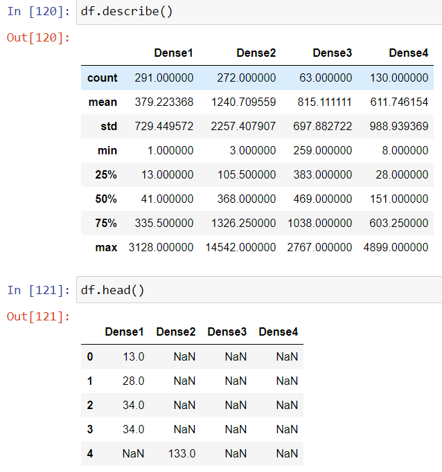
Let’s subset and rearrange the dataset that we can use for our ANOVA test:

df=pd.DataFrame({'Dense1':data[data['density_Group']=='Dense1']['Positive'],
                 'Dense2':data[data['density_Group']=='Dense2']['Positive'],
                 'Dense3':data[data['density_Group']=='Dense3']['Positive'],
                 'Dense4':data[data['density_Group']=='Dense4']['Positive']})

One of our ANOVA test’s assumptions is that samples should be randomly selected and should be close to Gaussian Distribution. So let’s select 10 random samples from each factor or level:

np.random.seed(1234)
dataNew=pd.DataFrame({'Dense1':random.sample(list(data['Positive'][data['density_Group']=='Dense1']), 10),
'Dense2':random.sample(list(data['Positive'][data['density_Group']=='Dense1']), 10),
'Dense3':random.sample(list(data['Positive'][data['density_Group']=='Dense1']), 10),
'Dense4':random.sample(list(data['Positive'][data['density_Group']=='Dense1']), 10)})

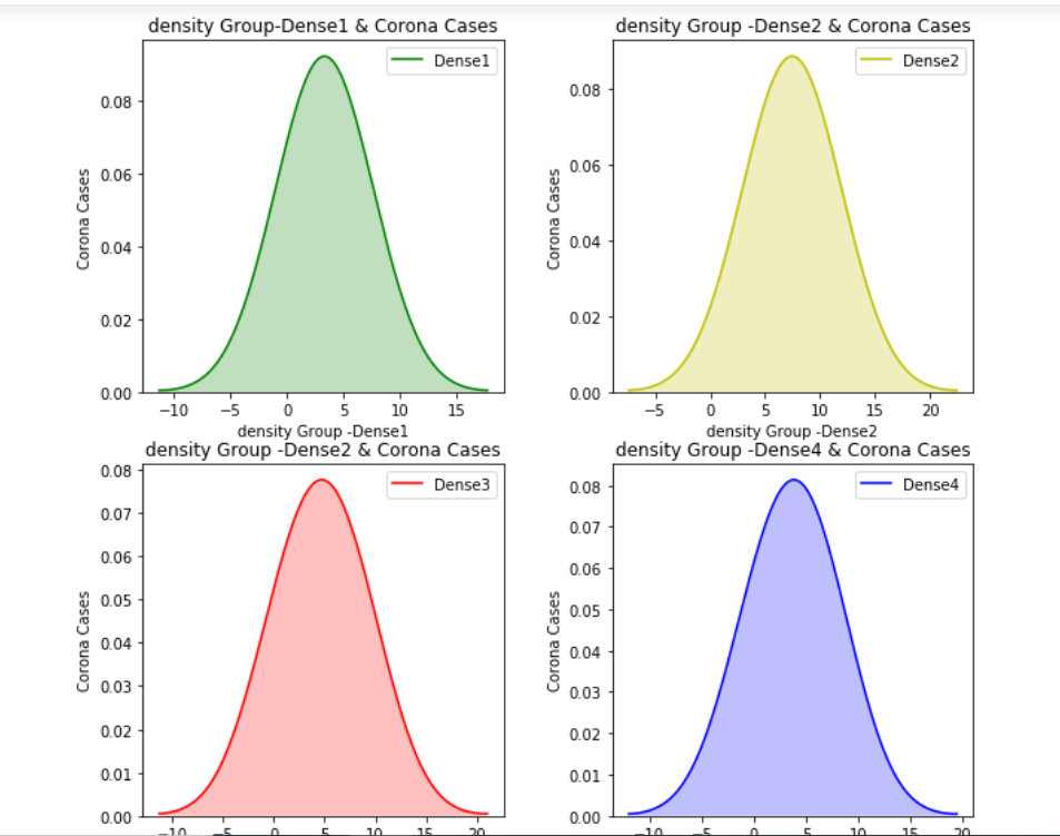
Let’s plot a density distribution of the number of Corona cases to check their distribution across different density groups:

We can clearly see that the data doesn’t follow the Gaussian distribution.

There are different data transformation methods available to bring the data to close to Gaussian Distribution. We’ll go ahead with Box Cox transformation:

dataNew['Dense1'],fitted_lambda = stats.boxcox(dataNew['Dense1'])
dataNew['Dense2'],fitted_lambda = stats.boxcox(dataNew['Dense2'])
dataNew['Dense3'],fitted_lambda = stats.boxcox(dataNew['Dense3'])
dataNew['Dense4'],fitted_lambda = stats.boxcox(dataNew['Dense4'])

Now let’s plot their distribution once again to check:

Approach 1: One-Way ANOVA Test using statsmodels module

There are a couple of methods in Python to perform an ANOVA test. One is with the stats.f_oneway() method:

F, p = stats.f_oneway(dataNew['Dense1'],dataNew['Dense2'],dataNew['Dense3'],dataNew['Dense4'])
# Seeing if the overall model is significant
print('F-Statistic=%.3f, p=%.3f' % (F, p))

We see that p-value <0.05. Hence, we can reject the Null Hypothesis – there are no differences among different density groups.

Approach 2: One-Way ANOVA Test using OLS Model

As we know in regression, we can regress against each input variable and check its influence over the Target variable. So, we’ll follow the same approach, the approach we follow in Linear Regression.

model = ols('Count ~ C(density_Group)', newDf).fit()
model.summary()

# Seeing if the overall model is significant
print(f"Overall model F({model.df_model: .0f},{model.df_resid: .0f}) = {model.fvalue: .3f}, p = {model.f_pvalue: .4f}")

# Creates the ANOVA table
res = sm.stats.anova_lm(model, typ= 2)
res

From the above output results, we see that the p-value is less than 0.05. Hence, we can reject the Null Hypothesis that there’s no difference among different density groups.

The F-statistic= 5.817 and the p-value= 0.002 which is indicating that there is an overall significant effect of density_Group on corona positive cases. However, we don’t know where the difference between desnity_groups is yet. So, based on the p-value we can reject the H0; that is there’s no significant difference as per density of an area and number of corona cases.

Post Hoc Tests

When we conduct an ANOVA, we are attempting to determine if there is a statistically significant difference among the groups. So what if we find statistical significance?

If we find that there is a difference, we will then need to examine where the group differences lay. So, we’ll use the Tukey HSD test to identify where the difference lies:

mc = statsmodels.stats.multicomp.MultiComparison(newDf['Count'],newDf['density_Group'])
mc_results = mc.tukeyhsd()
print(mc_results)

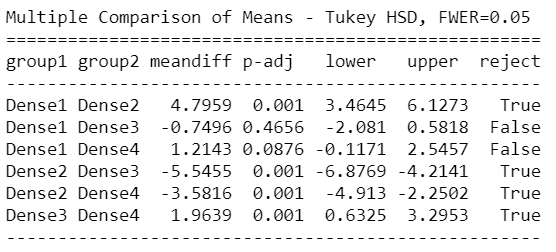
Tuckey HSD test clearly says that there’s a significant difference between Group1 – Group3 , Group1 – Group4, Group2 – Group3, and Group3 – Group4.

This suggests that except for the mentioned groups, all other pairwise comparisons for the number of Corona cases reject the null hypothesis and indicate no statistically significant differences.

Assumption Checks/Model Diagnostics

Normal Distribution Assumption check

When working with linear regression and ANOVA models, the assumptions pertain to the residuals and not the variables themselves.

Method 1: Shapiro Wilk test:

### Normality Assumption check
w, pvalue = stats.shapiro(model.resid)
print(w, pvalue)

From the above snippet of code, we see that the p-value is >0.05 for all density groups. Hence, we can conclude that they follow the Gaussian Distribution.

Method 2: Q-Q plot test:

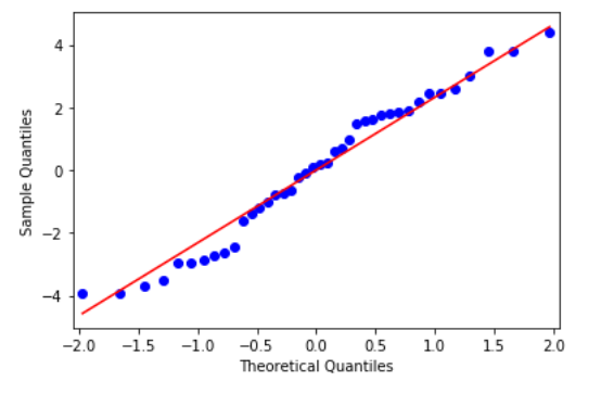
We can use the Normal Q-Q plot to test this assumption:

res = model.resid
fig = sm.qqplot(res, line='s')
plt.show()

From the above figure, we see that all data points lie to close to the 45-degree line and hence we can conclude that it follows Normal Distribution.

Homogeneity of Variance Assumption check

The homogeneity of variance assumption should be checked for each level of the categorical variable. We can use the Levene’s test to test for equal variances between groups.

w, pvalue = stats.bartlett(newDf['Count'][newDf['density_Group']=='Dense1'], newDf['Count'][newDf['density_Group']=='Dense2']
                           , newDf['Count'][newDf['density_Group']=='Dense3'], newDf['Count'][newDf['density_Group']=='Dense4'])
print(w, pvalue)

# Levene variance test, Method 2
stats.levene(dataNew['Dense1'],dataNew['Dense2'],dataNew['Dense3'],dataNew['Dense4'])

We see that p-value >0.05 for all density groups. Hence, we can conclude that groups have equal variances.

Two-Way ANOVA Test in Python

Again, using the same dataset, we’ll try to understand if there’s any significant relationship between the density of a region or state, age of people, and the number of corona cases. So, we’ll map each state according to the density of the population residing in it.

Let’s import the data and check if there’s any data ambiguity:

individualDetails=pd.read_csv('./individualDetails.csv',parse_dates=[2])
stateDensity=pd.read_csv('./stateDensity.csv')

From the above code snippet, we can see that there’s no record of an infected infant. Next, check for missing values in our data:

individualDetails.isna().sum()

print('Percentage of missing values in age & gender columns respectively :', \
      (individualDetails['age'].isna().sum()/individualDetails.shape[0])*100,'%',\
      (individualDetails['gender'].isna().sum()/individualDetails.shape[0])*100,'%')

We see that more than 91% and 80% entries are missing in the age & gender columns respectively. So we need to devise a method in order to impute them.

Here, I’ll impute age with the median value in each state and gender by mode of male & female in each state. So I’ll calculate median and mode:

ageMedianPerState=individualDetails[~individualDetails['age'].isna()]
ageMedianPerState['age']=ageMedianPerState['age'].astype(str).astype(int)
ageMedianPerState=ageMedianPerState.groupby('State')[['age']].median().reset_index()
ageMedianPerState['age']=ageMedianPerState['age'].apply(lambda x:math.ceil(x))

#Find the most frequent infected gender by COVID-19 for each state
genderModePerState=individualDetails.groupby(['State'])['gender'].agg(pd.Series.mode).to_frame().reset_index()

#Drop Arunachal Pradesh since this has got no informatio about gender overall
genderModePerState=genderModePerState[genderModePerState['State']!='Arunachal Pradesh']

#Impute missing values in age & gender columns now
for index,row in individualDetails.iterrows():
    if row['State']=='Arunachal Pradesh':    
        individualDetails.drop([index],inplace=True)
        continue
    if pd.isnull(row['age']):
        individualDetails['age'][index]=list(ageMedianPerState['age'][ageMedianPerState['State']=='West Bengal'].values)[0]
    if pd.isnull(row['gender']):
        if len(genderModePerState['gender'][genderModePerState['State']==row['State']].values)>0:
            individualDetails['gender'][index]=(genderModePerState['gender'][genderModePerState['State']==row['State']].values[0])

Now let’s merge individualDetails & stateDensity dataframe to create an overall dataset for us:

data = pd.merge(individualDetails,stateDensity,on='State',how='left').reset_index(drop=True)

Now we can create the age group bucket:

data.dropna(subset=['density_Group'],inplace=True)
data.reset_index(drop=True,inplace=True)

Merge the data to get a dataset with each person mapped with their age group and their respective state density group:

patient_Count=data.groupby(['diagnosed_date','density_Group'])[['diagnosed_date']].count().\

                        rename(columns={'diagnosed_date':'Count'}).reset_index()

data=pd.merge(data,patient_Count,on=['diagnosed_date','density_Group'],how='inner')




newData=data.groupby(['density_Group','age_Group'])['Count'].apply(list).reset_index()




newData.head()




np.random.seed(1234)

AnovaData=pd.DataFrame(columns=['density_Group','age_Group','Count'])

for index,row in newData.iterrows():

    count=17

    tempDf=pd.DataFrame(index=range(0,count),columns=['density_Group','age_Group','Count'])

   

    tempDf['age_Group']=newData['age_Group'][index]

    tempDf['density_Group']=newData['density_Group'][index]

    tempDf['Count']=random.sample(list(newData['Count'][index]),count)

    AnovaData=pd.concat([AnovaData,tempDf],axis=0)

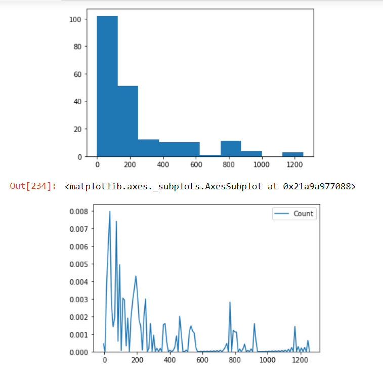
Check the distribution of the Count column in our data and check if there are outliers present in our data using the box plot method:

plt.hist(AnovaData['Count'])
plt.show() sns.kdeplot(AnovaData['Count'],cumulative=False,bw=2)

We see that there are many outliers present in our data. And even the distribution of the count variable is not Gaussian. So we’ll employ the Box-Cox transformation method to handle the situation:

sns.boxplot(x='age_Group', y='Count',
                 data=AnovaData,
                 palette="colorblind")

AnovaData['Count']=AnovaData['Count'].astype(int)

# Data Transformation
AnovaData['newCount'],fitted_lambda = stats.boxcox(AnovaData['Count'])

import matplotlib.pyplot as plt
sns.kdeplot(AnovaData['newCount'],cumulative=False,bw=2)

Now let’s employ the OLS model to check our Hypothesis:

# Fit the OlS model - Approach 1
model2 = ols('newCount ~ C(age_Group)+ C(density_Group)', AnovaData).fit()

print(f"Overall model F({model2.df_model: },{model2.df_resid: }) = {model2.fvalue: }, p = {model2.f_pvalue: }")
model2.summary()

# Create the ANOVA table
res2 = sm.stats.anova_lm(model2, typ=2)
res2

#Check the Normal distribution of residuals
res = model2.resid
fig = sm.qqplot(res, line='s')
plt.show()

From the above Q-Q plot, we can see that residuals are almost normally distributed (although points at the extreme ends can be discounted). Hence, we can conclude that it satisfies the Normality assumption of the ANOVA test.

#Approach 2 - Check the interaction of groups
formula = 'newCount ~ C(age_Group) *C(density_Group)'
model = ols(formula, AnovaData).fit()
model.summary()

aov_table = anova_lm(model, typ=2)
print(aov_table.round(4))

Interpretation of results

The P-value obtained from ANOVA analysis for the number of Corona cases, age group and density group and interaction are statistically significant (P < 0.05). We conclude that type of density_Group significantly affects the corona case outcome.

age_Group significantly affects the corona cases outcome, and interaction of both age_Group and density_Group significantly affects the corona case outcome as well.

Post Hoc Test

Finally, let’s identify which groups are statistically different. We’ll use the Tuckey HSD method for it:

mc = statsmodels.stats.multicomp.MultiComparison(AnovaData['newCount'],AnovaData['density_Group'])
mc_results = mc.tukeyhsd()
print(mc_results)

mc = statsmodels.stats.multicomp.MultiComparison(AnovaData['newCount'],AnovaData['age_Group'])
mc_results = mc.tukeyhsd()
print(mc_results)

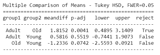
From the above Tuckey HSD test results, we can see clearly that there’s a significant difference between Group1 – Group3, Group1 – Group4 in density groups, and Young – Adult & Young – old groups in the age group as well.

So the above result from Tukey HSD suggests that except for the mentioned groups, all other pairwise comparisons for the number of Corona cases reject the null hypothesis and indicate no statistically significant differences.

End Notes

I’ve tried my bit to explain the ANOVA test using a relevant case study in these pandemic times. It was a fun experience putting this all together for our community!

Please feel free to comment below with your queries and I’ll be more than happy to answer. You can clone my Github repository to download the whole code & data here!

About the Author

Praveen Kumar Anwla

I’ve been working as a Data Scientist with product-based and Big 4 Audit companies for almost 5 years now. I have been working on various NLP, machine learning & cutting edge deep learning business problems. Please feel free to check out my personal blog where I cover topics from Machine learning – AI to Visualization tools ( Tableau, QlikView, etc.) & various cloud platforms like Azure, IBM & AWS cloud.