This is the end of this blog. Let me know if you have any suggestions/doubts.
Find the Python notebook with the entire code along with the dataset and all the illustrations here.
Let me know how you found this blog 🙂
Recommendation systems are becoming increasingly important in today’s hectic world. People are always in the lookout for products/services that are best suited for them. Therefore, the recommendation systems are important as they help them make the right choices, without having to expend their cognitive resources. In this blog, we will understand the basics of knn recommender system and learn how to build a Movie Recommendation System using collaborative filtering by implementing the K-Nearest Neighbors algorithm. We will also predict the rating of the given movie based on its neighbors and compare it with the actual rating.
Recommendation systems can be broadly classified into 3 types —
This filtering method is usually based on collecting and analyzing information on user’s behaviors, their activities or preferences, and predicting what they will like based on the similarity with other users. A key advantage of the collaborative filtering approach is that it does not rely on machine analyzable content and thus it is capable of accurately recommending complex items such as movies without requiring an “understanding” of the item itself.
Further, there are several types of collaborative filtering algorithms —
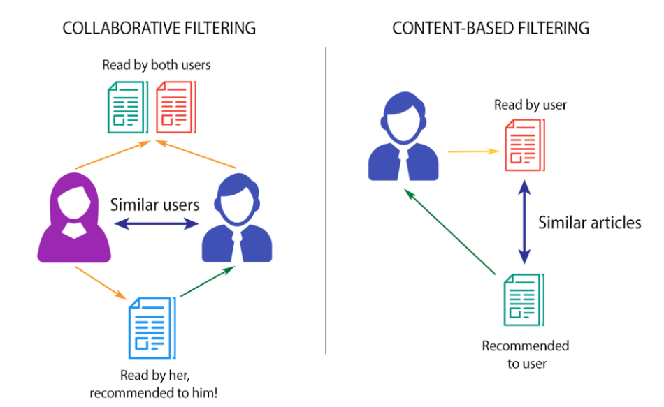
These filtering methods are based on the description of an item and a profile of the user’s preferred choices. In a content-based recommendation system, keywords are used to describe the items, besides, a user profile is built to state the type of item this user likes. In other words, the algorithms try to recommend products that are similar to the ones that a user has liked in the past.
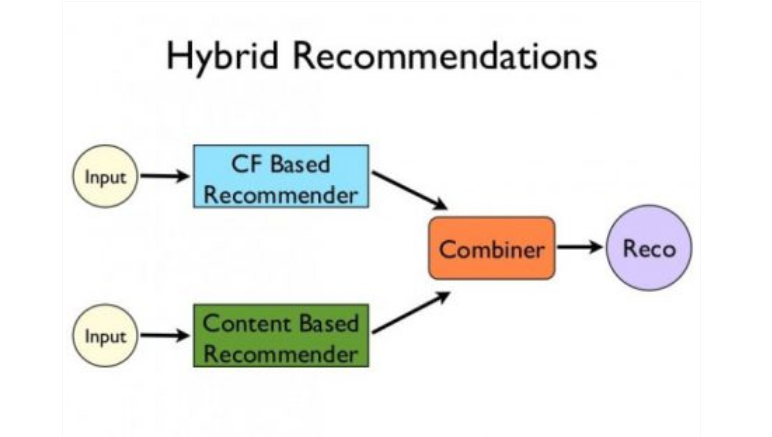
Recent research has demonstrated that a hybrid approach, combining collaborative filtering and content-based filtering could be more effective in some cases. Hybrid approaches can be implemented in several ways, by making content-based and collaborative-based predictions separately and then combining them, by adding content-based capabilities to a collaborative-based approach (and vice versa), or by unifying the approaches into one model.
Netflix is a good example of the use of hybrid recommender systems. The website makes recommendations by comparing the watching and searching habits of similar users (i.e. collaborative filtering) as well as by offering movies that share characteristics with films that a user has rated highly (content-based filtering).
Now that we’ve got a basic intuition of Recommendation Systems, let’s start with building a simple Movie Recommendation System in Python.
Find the Python notebook with the entire code along with the dataset and all the illustrations here.
The Movie Database (TMDb) is a community built movie and TV database which has extensive data about movies and TV Shows. Here are the stats —

For simplicity and easy computation, I have used a subset of this huge dataset which is the TMDb 5000 dataset. It has information about 5000 movies, split into 2 CSV files.
The link to the Dataset is here.
Import the required Python libraries like Pandas, Numpy, Seaborn, and Matplotlib. Then import the CSV files using read_csv() function predefined in Pandas.
movies = pd.read_csv('../input/tmdb-movie-metadata/tmdb_5000_movies.csv')
credits = pd.read_csv('../input/tmdb-movie-metadata/tmdb_5000_credits.csv')
We will initially use the head(), describe() function to view the values and structure of the dataset, and then move ahead with cleaning the data.
movies.head()
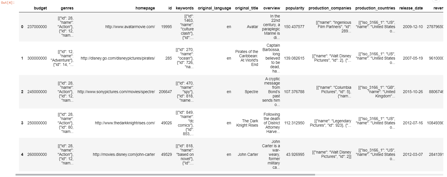
Python Code:
import pandas as pd

# Reading the data
movies = pd.read_csv('tmdb_5000_movies.csv')

# Head and describe
print(movies.head())
print('______________________________')
print(movies.describe())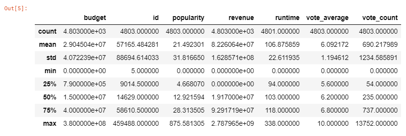
Similarly, we can get an intuition of the credits dataframe and get an output as follows —

Checking the dataset, we can see that genres, keywords, production_companies, production_countries, spoken_languages are in the JSON format. Similarly in the other CSV file, cast and crew are in the JSON format. Now let’s convert these columns into a format that can be easily read and interpreted. We will convert them into strings and later convert them into lists for easier interpretation.
The JSON format is like a dictionary (key: value) pair embedded in a string. Generally, parsing the data is computationally expensive and time-consuming. Luckily this dataset doesn’t have that complicated structure. A basic similarity between the columns is that they have a name key, which contains the values that we need to collect. The easiest way to do so parse through the JSON and check for the name key on each row. Once the name key is found, store the value of it into a list and replace the JSON with the list.
But we cannot directly parse this JSON as it has to be decoded first. For this, we use the json.loads() method, which decodes it into a list. We can then parse through this list to find the desired values. Let’s look at the proper syntax below.
# changing the genres column from json to string
movies['genres'] = movies['genres'].apply(json.loads)
for index,i in zip(movies.index,movies['genres']):
    list1 = []
    for j in range(len(i)):
        list1.append((i[j]['name'])) # the key 'name' contains the name of the genre
    movies.loc[index,'genres'] = str(list1)
In a similar fashion, we will convert the JSON to a list of strings for the columns: keywords, production_companies, cast, and crew. We will check if all the required JSON columns have been converted to strings using movies.iloc[index]
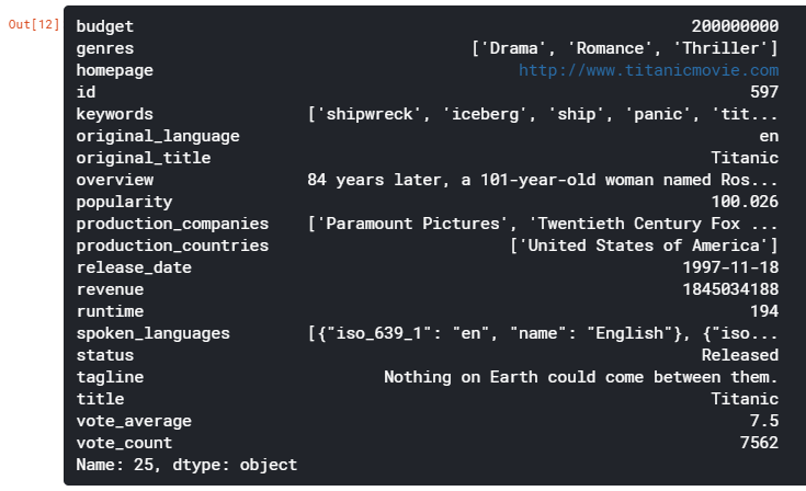
We will merge the movies and credits dataframes and select the columns which are required and have a unified movies dataframe to work on.
movies = movies.merge(credits, left_on='id', right_on='movie_id', how='left')
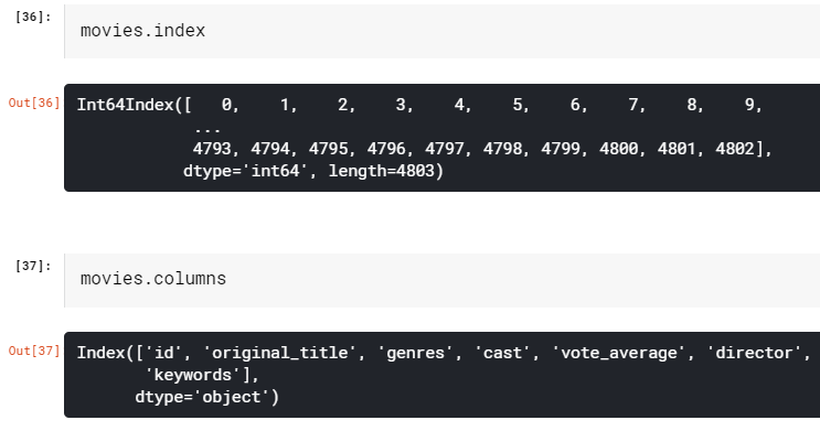
movies = movies[['id', 'original_title', 'genres', 'cast', 'vote_average', 'director', 'keywords']]
We can check the size and attributes of movies like this —
We will clean the genre column to find the genre_list
movies['genres'] = movies['genres'].str.strip('[]').str.replace(' ','').str.replace("'",'')
movies['genres'] = movies['genres'].str.split(',')
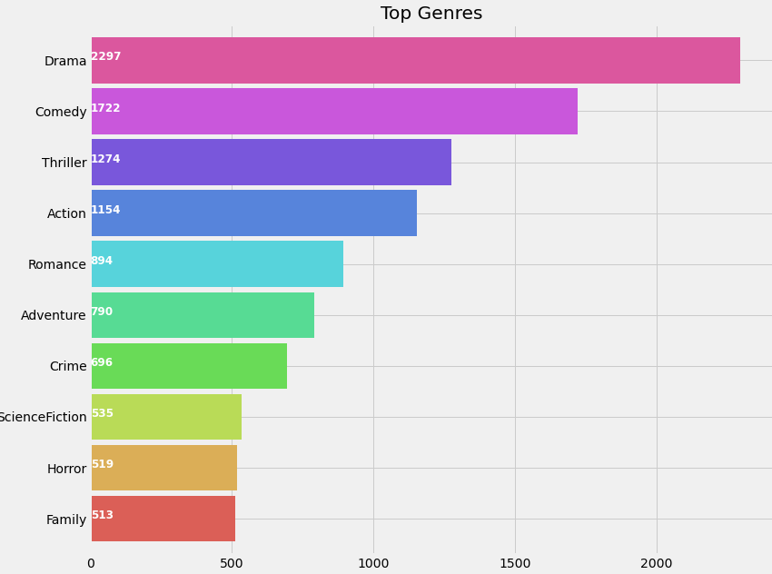
Let’s plot the genres in terms of their occurrence to get an insight into movie genres in terms of popularity.
plt.subplots(figsize=(12,10))
list1 = []
for i in movies['genres']:
    list1.extend(i)
ax = pd.Series(list1).value_counts()[:10].sort_values(ascending=True).plot.barh(width=0.9,color=sns.color_palette('hls',10))
for i, v in enumerate(pd.Series(list1).value_counts()[:10].sort_values(ascending=True).values):
    ax.text(.8, i, v,fontsize=12,color='white',weight='bold')
plt.title('Top Genres')
plt.show()
Now let’s generate a list ‘genreList’ with all possible unique genres mentioned in the dataset.
genreList = []
for index, row in movies.iterrows():
    genres = row["genres"]

    for genre in genres:
        if genre not in genreList:
            genreList.append(genre)
genreList[:10] #now we have a list with unique genres
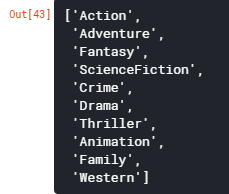
‘genreList’ will now hold all the genres. But how do we come to know about the genres each movie falls into. Now some movies will be ‘Action’, some will be ‘Action, Adventure’, etc. We need to classify the movies according to their genres.
Let’s create a new column in the dataframe that will hold the binary values whether a genre is present or not in it. First, let’s create a method that will return back a list of binary values for the genres of each movie. The ‘genreList’ will be useful now to compare against the values.
Let’s say for example we have 20 unique genres in the list. Thus the below function will return a list with 20 elements, which will be either 0 or 1. Now for example we have a Movie which has genre = ‘Action’, then the new column will hold [1,0,0,0,0,0,0,0,0,0,0,0,0,0,0,0,0,0,0,0].
Similarly for ‘Action, Adventure’ we will have, [1,1,0,0,0,0,0,0,0,0,0,0,0,0,0,0,0,0,0,0]. Converting the genres into such a list of binary values will help in easily classifying the movies by their genres.
def binary(genre_list):
    binaryList = []

    for genre in genreList:
        if genre in genre_list:
            binaryList.append(1)
        else:
            binaryList.append(0)

    return binaryList
Applying the binary() function to the ‘genres’ column to get ‘genre_list’
We will follow the same notations for other features like the cast, director, and the keywords.
movies['genres_bin'] = movies['genres'].apply(lambda x: binary(x))
movies['genres_bin'].head()

Let’s plot a graph of Actors with Highest Appearances
plt.subplots(figsize=(12,10))
list1=[]
for i in movies['cast']:
    list1.extend(i)
ax=pd.Series(list1).value_counts()[:15].sort_values(ascending=True).plot.barh(width=0.9,color=sns.color_palette('muted',40))
for i, v in enumerate(pd.Series(list1).value_counts()[:15].sort_values(ascending=True).values):
    ax.text(.8, i, v,fontsize=10,color='white',weight='bold')
plt.title('Actors with highest appearance')
plt.show()
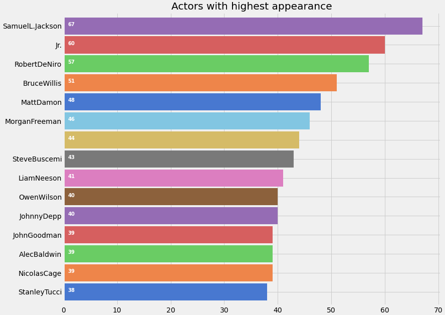
Samuel Jackson aka Nick Fury from Avengers has appeared in maximum movies. I initially thought that Morgan Freeman might be the actor with maximum movies, but Data wins over assumptions!
When I initially created the list of all the cast, it had around 50k unique values, as many movies have entries for about 15–20 actors. But do we need all of them? The answer is No. We just need the actors who have the highest contribution to the movie. For eg: The Dark Knight franchise has many actors involved in the movie. But we will select only the main actors like Christian Bale, Micheal Caine, Heath Ledger. I have selected the main 4 actors from each movie.
One question that may arise in your mind is how do you determine the importance of the actor in the movie. Luckily, the sequence of the actors in the JSON format is according to the actor’s contribution to the movie.
Let’s see how we do that and create a column ‘cast_bin’
for i,j in zip(movies['cast'],movies.index):
    list2 = []
    list2 = i[:4]
    movies.loc[j,'cast'] = str(list2)
movies['cast'] = movies['cast'].str.strip('[]').str.replace(' ','').str.replace("'",'')
movies['cast'] = movies['cast'].str.split(',')
for i,j in zip(movies['cast'],movies.index):
    list2 = []
    list2 = i
    list2.sort()
    movies.loc[j,'cast'] = str(list2)
movies['cast']=movies['cast'].str.strip('[]').str.replace(' ','').str.replace("'",'')castList = []
for index, row in movies.iterrows():
    cast = row["cast"]

    for i in cast:
        if i not in castList:
            castList.append(i)movies[‘cast_bin’] = movies[‘cast’].apply(lambda x: binary(x))
movies[‘cast_bin’].head()

Let’s plot Directors with maximum movies
def xstr(s):
    if s is None:
        return ''
    return str(s)
movies['director'] = movies['director'].apply(xstr)plt.subplots(figsize=(12,10))
ax = movies[movies['director']!=''].director.value_counts()[:10].sort_values(ascending=True).plot.barh(width=0.9,color=sns.color_palette('muted',40))
for i, v in enumerate(movies[movies['director']!=''].director.value_counts()[:10].sort_values(ascending=True).values):
    ax.text(.5, i, v,fontsize=12,color='white',weight='bold')
plt.title('Directors with highest movies')
plt.show()
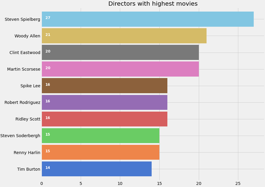
We create a new column ‘director_bin’ as we have done earlier
directorList=[]
for i in movies['director']:
    if i not in directorList:
        directorList.append(i)movies['director_bin'] = movies['director'].apply(lambda x: binary(x))
movies.head()
So finally, after all this work we get the movies dataset as follows

The keywords or tags contain a lot of information about the movie, and it is a key feature in finding similar movies. For eg: Movies like “Avengers” and “Ant-man” may have common keywords like superheroes or Marvel.
For analyzing keywords, we will try something different and plot a word cloud to get a better intuition:
from wordcloud import WordCloud, STOPWORDS
import nltk
from nltk.corpus import stopwordsplt.subplots(figsize=(12,12))
stop_words = set(stopwords.words('english'))
stop_words.update(',',';','!','?','.','(',')','

We find ‘words_bin’ from Keywords as follows —
movies['keywords'] = movies['keywords'].str.strip('[]').str.replace(' ','').str.replace("'",'').str.replace('"','')
movies['keywords'] = movies['keywords'].str.split(',')
for i,j in zip(movies['keywords'],movies.index):
    list2 = []
    list2 = i
    movies.loc[j,'keywords'] = str(list2)
movies['keywords'] = movies['keywords'].str.strip('[]').str.replace(' ','').str.replace("'",'')
movies['keywords'] = movies['keywords'].str.split(',')
for i,j in zip(movies['keywords'],movies.index):
    list2 = []
    list2 = i
    list2.sort()
    movies.loc[j,'keywords'] = str(list2)
movies['keywords'] = movies['keywords'].str.strip('[]').str.replace(' ','').str.replace("'",'')
movies['keywords'] = movies['keywords'].str.split(',')words_list = []
for index, row in movies.iterrows():
    genres = row["keywords"]

    for genre in genres:
        if genre not in words_list:
            words_list.append(genre)movies['words_bin'] = movies['keywords'].apply(lambda x: binary(x))
movies = movies[(movies['vote_average']!=0)] #removing the movies with 0 score and without drector names
movies = movies[movies['director']!='']
We will be using Cosine Similarity for finding the similarity between 2 movies. How does cosine similarity work?
Let’s say we have 2 vectors. If the vectors are close to parallel, i.e. angle between the vectors is 0, then we can say that both of them are “similar”, as cos(0)=1. Whereas if the vectors are orthogonal, then we can say that they are independent or NOT “similar”, as cos(90)=0.
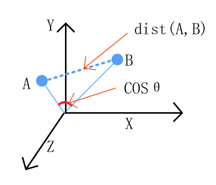
For a more detailed study, follow this link.
Below I have defined a function Similarity, which will check the similarity between the movies.
from scipy import spatialdef Similarity(movieId1, movieId2):
    a = movies.iloc[movieId1]
    b = movies.iloc[movieId2]

    genresA = a['genres_bin']
    genresB = b['genres_bin']

    genreDistance = spatial.distance.cosine(genresA, genresB)

    scoreA = a['cast_bin']
    scoreB = b['cast_bin']
    scoreDistance = spatial.distance.cosine(scoreA, scoreB)

    directA = a['director_bin']
    directB = b['director_bin']
    directDistance = spatial.distance.cosine(directA, directB)

    wordsA = a['words_bin']
    wordsB = b['words_bin']
    wordsDistance = spatial.distance.cosine(directA, directB)
    return genreDistance + directDistance + scoreDistance + wordsDistance
Let’s check the Similarity between 2 random movies

We see that the distance is about 2.068, which is high. The more the distance, the less similar the movies are. Let’s see what these random movies actually were.
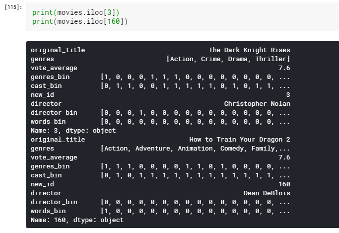
It is evident that The Dark Knight Rises and How to train your Dragon 2 are very different movies. Thus the distance is huge.
So now when we have everything in place, we will now build the score predictor. The main function working under the hood will be the Similarity() function, which will calculate the similarity between movies, and will find 10 most similar movies. These 10 movies will help in predicting the score for our desired movie. We will take the average of the scores of similar movies and find the score for the desired movie.
Now the similarity between the movies will depend on our newly created columns containing binary lists. We know that features like the director or the cast will play a very important role in the movie’s success. We always assume that movies from David Fincher or Chris Nolan will fare very well. Also if they work with their favorite actors, who always fetch them success and also work on their favorite genres, then the chances of success are even higher. Using these phenomena, let’s try building our score predictor.
import operatordef predict_score():
    name = input('Enter a movie title: ')
    new_movie = movies[movies['original_title'].str.contains(name)].iloc[0].to_frame().T
    print('Selected Movie: ',new_movie.original_title.values[0])
    def getNeighbors(baseMovie, K):
        distances = []

        for index, movie in movies.iterrows():
            if movie['new_id'] != baseMovie['new_id'].values[0]:
                dist = Similarity(baseMovie['new_id'].values[0], movie['new_id'])
                distances.append((movie['new_id'], dist))

        distances.sort(key=operator.itemgetter(1))
        neighbors = []

        for x in range(K):
            neighbors.append(distances[x])
        return neighbors

    K = 10
    avgRating = 0
    neighbors = getNeighbors(new_movie, K)print('\nRecommended Movies: \n')
    for neighbor in neighbors:
        avgRating = avgRating+movies.iloc[neighbor[0]][2]
        print( movies.iloc[neighbor[0]][0]+" | Genres: "+str(movies.iloc[neighbor[0]][1]).strip('[]').replace(' ','')+" | Rating: "+str(movies.iloc[neighbor[0]][2]))

    print('\n')
    avgRating = avgRating/K
    print('The predicted rating for %s is: %f' %(new_movie['original_title'].values[0],avgRating))
    print('The actual rating for %s is %f' %(new_movie['original_title'].values[0],new_movie['vote_average']))
Now simply just run the function as follows and enter the movie you like to find 10 similar movies and it’s predicted ratings
predict_score()

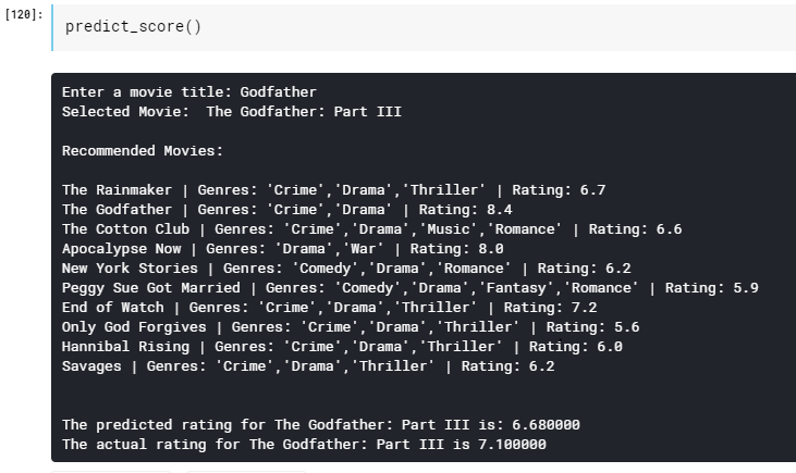
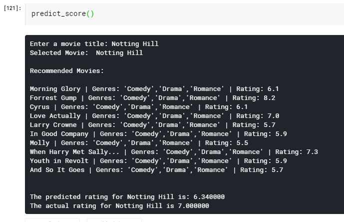
Thus we have completed the Movie Recommendation System implementation using the K-Nearest Neighbors algorithm.
In this project, we have arbitrarily chosen the value K=10.
But in other applications of KNN, finding the value of K is not easy. A small value of K means that noise will have a higher influence on the result and a large value make it computationally expensive. Data scientists usually choose as an odd number if the number of classes is 2 and another simple approach to select k is set K=sqrt(n).
This is the end of this blog. Let me know if you have any suggestions/doubts.
Find the Python notebook with the entire code along with the dataset and all the illustrations here.
Let me know how you found this blog 🙂
Check out – Future of AI and ML in the Next 10 Years
kNN algorithm is a reliable and intuitive recommendation system that leverages user or item similarity to provide personalized recommendations. kNN recommender system is helpful in e-commerce, social media, and healthcare, and continues to be an important tool for generating accurate and personalized recommendations.
Thanks for walking through K-means approach, Heeral. It's interesting to see even this algorithm can be used for recommender systems. I see two parts: one is the 10 closest movies and the other is the rating prediction at the end of your analysis. Out of reading about the connection between predicting the rating and making recommendations, I would like to understand 'why is the rating even predicted' when we want the most similar items to a movie or an item? And getting the 10 most similar items is always possible with a wide variety of similarity techniques out there.
Hey Akshay, the rating prediction was an add-on thing with the recommendation part. I implemented the rating prediction to check if the similar items were in the same range as the main item in terms of rating. If the difference is too big then there is something which is not considered and the system is giving erroneous results. Yes, I am aware about the various similarity techniques out there, Cosine Similarity is a rather easy to understand and is a fundamental technique.
Hey Akshay, the rating prediction was an additional thing to the recommendation system. Idea behind it was to check that the recommendations are not too far away from the original item in terms of rating. If the difference is big, it means we missed out on considering something. Yes, I am aware of other techniques used in Recommendation Algorithms, but Cosine Similarity is rather easy-to-understand and is a fundamental Similarity technique.
Hey Akshay, thank you for your feedback. The idea behind Rating Prediction was to verify that the movies that are recommended are in the same range as the primary movie in terms of ratings. If the difference between predicted and actual rating is too much, it means that the recommendations are not correctly attributed. I believe we could do more with the rating prediction alone by using different Machine Learning algorithms, but that would be a different project altogether. Yes, I am aware of other similarity techniques out there, I chose Cosine Similarity because it is easy-to-understand and is a fundamental technique.
I still confuse with different between Item-Item Collaborative Filtering with conten base filtering.
Hello DATNGUYEN, in Item-Item Collaborative Filtering you are talking about getting recommendations of the "items which are similar" to the item you are looking at. On the other hand, Content Based Filtering uses keywords used to describe the product along with the user profile who is searching it to give recommendations. Consider the item to be a Toothbrush. In Item-Item Collaborative Filtering you would get recommendations of brushes of other brands, whereas in Content Based Filtering you would a suggestion of a Toothpaste, or dental floss. Hope that helps :)
Hey DAITNGUYEN, in Item-Item Collaborative Filtering the recommendations are solely based on items which are similar to the current item. On the other hand, in Content Based Filtering, the recommendations are based on the keywords used to describe the product as well as the previous profile of the user. For example, if the current item is a toothbrush, in Item-Item Collaborative Filtering you will get a recommendation of a toothbrush from another brand; whereas in Content Based Filtering, you will get the recommendation of a toothpaste because they will have similar keywords.
Hi, I tried out your code and actually understood most of it. Thanks! But towards the end, it says the variable 'new_id' is not found. I was not able to figure out where exactly we defined it. It would be great if you could help.