Introduction
In general terms, this article is going to be about data cleansing. Specifically, the process I would like to explore is actually a small subset of the cleansing process: Merging disparate data sources on common categories.
A quick primer on data cleansing (you can skip this if you are familiar)
Data cleansing is a highly important task that you should take absolutely seriously. I’ve seen countless data specialists joke that their jobs essentially boil down to being a glorified data janitor, doomed to mop the floors in the Hall of Records of the Hopper School of Data after perpetual problem children spill every sticky thing they can get their hands on. Okay, I may have some liberties with the metaphor; The point is that data cleansing is important and you are within your rights to call yourself a data janitor if the shoe fits.
Data cleansing is often the crux of the analytic process. All downstream processes are contingent on the output of this step. There are varying degrees of how much cleansing is necessary, but you should be at least comfortable with the process. Data cleaning is the process of fixing or removing incorrect, corrupted, incorrectly formatted, duplicate, or incomplete data within a dataset (source: https://www.tableau.com/learn/articles/what-is-data-cleaning).
Merging data sources
When combining data from multiple sources there is often a lot of issues to correct for. Different sources will often have different naming conventions than your main source, different ways of grouping data, etc. Most of the time the additional data source was created at a much different point in time, by different engineers and stakeholders, and (almost) always with different goals and use-cases. In light of this, it shouldn’t be surprising to encounter a wide array of differences between multiple sources.
Here I would like to explore various ways of simplifying (hopefully) the merging process in a way that delivers concrete value to downstream users. There are many use cases where this could be of value. For example: If you have two systems that operate in parallel to each other and you need to perform some analysis of the relationship, you have a legacy system with poorly formatted data that needs to be integrated into a crisp new system, etc. The example I would like to dive into is the analysis of parallel systems.
Analysis of parallel systems
This is a surprisingly common problem with organizations that use dated systems and software. What often happens is that additional needs arise that are not being met by the legacy system, and the organization will commission a new tool or subscribe to a service that only provides a solution to the gap left by the legacy system. Eventually, this leads to the organization using a system from the early ’90s, supplemented by additional systems from each subsequent decade. While some of these systems are likely independent of each other, there are potentially valuable insights that could be earned from analyzing the data as a whole.
When approached by stakeholders to solve this problem, a common solution that is proposed is the creation of some type of mapping table that can be used to perform the joins. This is not a bad solution granted there is a clearly defined and close-ended mapping. More often, however, there will be mappings that were not foreseen when the mapping is created and potentially compounded by fields that are user-generated (yikes, I know). This makes a mapping table feasible when the stakeholders or end-users (read: people who don’t want more work) are responsible for the maintenance of this mapping, and they may try to pass this responsibility to you. The last thing you want is to be in charge of updating some obscure domain-specific mapping table; It’s not a good end result for anybody involved.
With this in mind, let’s try to explore some solutions. For the purposes of this exploration, I am going to consider anything that could potentially assist this process as a solution, even if it doesn’t solve the problem completely.
First, some data
I will create two distinct lists of names. One will be a clean set of standardized names, representing your main data source. The other will be a messy, jumbled, and inconsistent list representing the proverbial child spilling soda on the floor.
from random import random as rd
from random import randint as ri
from string import ascii_letters,ascii_lowercase

key_set = ['Terran','Protoss','Zerg']
idx = lambda X: ri(0,X)

mr_clean = [key_set[idx(2)] for x in range(5000)]
bad_child = [
    X + ''.join(
        [ascii_letters[idx(len(ascii_letters)-1)] for x in range(idx(15))]
        ) for X in mr_clean
    ]

print(mr_clean[:3])
print(bad_child[:3])['Zerg', 'Terran', 'Terran']
['ZergIeLZV', 'Terran', 'TerranszyvrRoxKGgzV']
To create the messy dataset, I’ve added a random number of random ascii characters to the end of each element from the clean list.
Candidate 1: Clustering
The first step here is to transform the letters for each element into more useful representation. To accomplish this, we’ll use sklearn’s CountVectorizer to transform the words into a matrix of character counts.
from sklearn.feature_extraction.text import CountVectorizer as CV
corpus = list(ascii_lowercase)
vec = CV(vocabulary=corpus,analyzer='char')

mr_clean_vec = [x.lower() for x in mr_clean]
bad_child_vec = [x.lower() for x in bad_child]

mr_clean_vec = vec.fit_transform(mr_clean_vec).toarray()
bad_child_vec = vec.fit_transform(bad_child_vec).toarray()

print(mr_clean_vec[:3])
print(bad_child_vec[:3])[[0 0 0 0 1 0 1 0 0 0 0 0 0 0 0 0 0 1 0 0 0 0 0 0 0 1]
 [1 0 0 0 1 0 0 0 0 0 0 0 0 1 0 0 0 2 0 1 0 0 0 0 0 0]
 [1 0 0 0 1 0 0 0 0 0 0 0 0 1 0 0 0 2 0 1 0 0 0 0 0 0]]
[[0 0 0 0 2 0 1 0 1 0 0 1 0 0 0 0 0 1 0 0 0 1 0 0 0 2]
 [1 0 0 0 1 0 0 0 0 0 0 0 0 1 0 0 0 2 0 1 0 0 0 0 0 0]
 [1 0 0 0 1 0 2 0 0 0 1 0 0 1 1 0 0 4 1 1 0 2 0 1 1 2]]
Now that the data is in an appropriate format, we can try clustering the output. In this case, because we are working with categorical variables we will use kmodes as opposed to kmeans. Kmeans uses Euclidean distance, which is not meaningful for categorical variables. First, I will test out kmodes using the clean data as a control to see how well it works for our purpose.
from kmodes.kmodes import KModes
import matplotlib.pyplot as plt
import seaborn as sns

kmodes = KModes(
    n_clusters=3, init = "Cao", n_init = 1, verbose=1
)
results = kmodes.fit_predict(mr_clean_vec)Init: initializing centroids
Init: initializing clusters
Starting iterations...
Run 1, iteration: 1/0, moves: 0, cost: 0.0import pandas as pd
clean_df = pd.DataFrame()
clean_df['labels'] = mr_clean
clean_df['kmodes'] = resultsplt.subplots(figsize = (5,5))
sns.countplot(
    x=clean_df['labels'],
    order=clean_df['labels'].value_counts().index,
    hue=clean_df['kmodes']
)
plt.show()
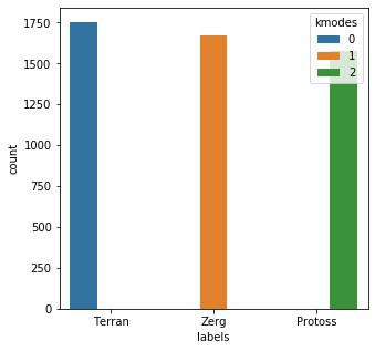
Based on the results chart, we can create a quick lookup dictionary to label and check the output.
lkup = {0:'Terran',1:'Zerg',2:'Protoss'}
clean_df['km_res'] = [lkup[x] for x in results]
clean_df['km_eval'] = clean_df['labels'] == clean_df['km_res']
clean_df.head()

clean_df['km_eval'].describe()count     5000
unique       1
top       True
freq      5000
Name: km_eval, dtype: object
For the clean dataset, kmodes selected the appropriate cluster 5000 of 5000 times. The control test appears to have been successful, so let’s try it on the soda-soaked list.
results = kmodes.fit_predict(bad_child_vec)
messy_df = pd.DataFrame()
messy_df['labels'] = mr_clean
messy_df['kmodes'] = results

plt.subplots(figsize = (5,5))
sns.countplot(
    x=messy_df['labels'],
    order=messy_df['labels'].value_counts().index,
    hue=messy_df['kmodes']
)
plt.show()Init: initializing centroids
Init: initializing clusters
Starting iterations...
Run 1, iteration: 1/100, moves: 1861, cost: 31942.0
Run 1, iteration: 2/100, moves: 1376, cost: 31050.0
Run 1, iteration: 3/100, moves: 2, cost: 31050.0
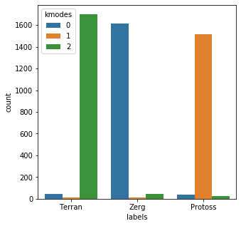
Okay so there’s a little more variety here, but overall it looks like there’s a solid mapping to draw from.
lkup = {0:'Zerg',1:'Protoss',2:'Terran'}
messy_df['km_res'] = [lkup[x] for x in results]
messy_df['km_eval'] = messy_df['labels'] == messy_df['km_res']
messy_df.head()

messy_df['km_eval'].describe()count     5000
unique       2
top       True
freq      4828
Name: km_eval, dtype: object
It looks like kmodes correctly grouped the categories in 4828/5000 tries, for a success rate of 96.56%. Not bad overall. One note of caution here is that this artificially messy data I created is not all that realistic. Since I simply tacked on a bunch of random garbage to the end of the category, at this point you could simply do this:
cleanup = [y for x in bad_child for y in key_set if y in x]

from collections import Counter
Counter([a==b for a,b in zip(mr_clean,cleanup)])[True]5000
Simply checking if the key string is found within the messy data solves the problem completely. In reality, this is not likely to be true. Let’s see if we can come up with something a bit more realistic.
from math import ceil

def css(word):
    noise = ceil(.3 * len(word)) # introduce a reasonable threshold of noise for the word
    mx = len(word)-1
    for _ in range(idx(noise)): # randomly add n characters
        pt = idx(mx)
        word = word[:pt] + ascii_letters[idx(len(ascii_letters)-1)] + word[pt:]
    return word

bad_child = [css(x) for x in mr_clean]
print(bad_child[:5])['YZNerg', 'dTebrran', 'Terran', 'Zervg', 'Protoss']
This introduces more realistic spelling and key errors into the messy dataset, so now let’s try kmodes again with our new noise.
bad_child_vec = [x.lower() for x in bad_child]
bad_child_vec = vec.fit_transform(bad_child_vec).toarray()

results = kmodes.fit_predict(bad_child_vec)
messy_df = pd.DataFrame()
messy_df['labels'] = mr_clean
messy_df['kmodes'] = results

plt.subplots(figsize = (5,5))
sns.countplot(
    x=messy_df['labels'],
    order=messy_df['labels'].value_counts().index,
    hue=messy_df['kmodes']
)
plt.show()Init: initializing centroids
Init: initializing clusters
Starting iterations...
Run 1, iteration: 1/100, moves: 130, cost: 5686.0
Run 1, iteration: 2/100, moves: 0, cost: 5686.0
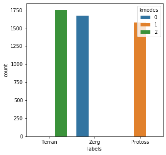
The output here actually looks very promising.
lkup = {0:'Zerg',1:'Protoss',2:'Terran'}
messy_df['km_res'] = [lkup[x] for x in results]
messy_df['km_eval'] = messy_df['labels'] == messy_df['km_res']
messy_df.head()

messy_df['km_eval'].describe()count     5000
unique       1
top       True
freq      5000
Name: km_eval, dtype: object
So this actually worked rather well; Each of the items, in this case, were classified correctly.
One of the drawbacks of a manual entry system, where you have humans inserting records, is that you are going to have human mistakes. There will be inconsistencies, misspellings, conflated terms, etc.; We will have to be able to account for these issues. Let’s introduce a little more complexity and add some inconsistencies.
junk = ['Industries','Ind','Inc','Co','Corp','Llc','Company']

bad_child = [css(x) for x in mr_clean]
bad_child = [x + ' ' + junk[idx(len(junk)-1)] for x in bad_child]

bad_child_vec = [x.lower() for x in bad_child]
bad_child_vec = vec.fit_transform(bad_child_vec).toarray()

results = kmodes.fit_predict(bad_child_vec)
messy_df = pd.DataFrame()
messy_df['labels'] = mr_clean
messy_df['kmodes'] = results

plt.subplots(figsize = (5,5))
sns.countplot(
    x=messy_df['labels'],
    order=messy_df['labels'].value_counts().index,
    hue=messy_df['kmodes']
)
plt.show()Init: initializing centroids
Init: initializing clusters
Starting iterations...
Run 1, iteration: 1/100, moves: 451, cost: 23933.0
Run 1, iteration: 2/100, moves: 0, cost: 23933.0
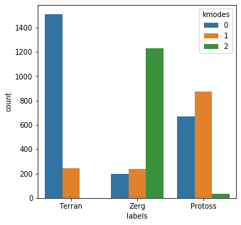
That’s more like it. Now we appear to have a real problem on our hands. Two of the categories were handled reasonably well, but the third category seems to be close to a near coin-flip result.
lkup = {0:'Terran',1:'Protoss',2:'Zerg'}
messy_df['km_res'] = [lkup[x] for x in results]
messy_df['km_eval'] = messy_df['labels'] == messy_df['km_res']
messy_df.head()

messy_df['km_eval'].describe()count     5000
unique       2
top       True
freq      3616
Name: km_eval, dtype: object
Clearly the results are less favorable now; 27.68% of the records are now mislabeled. The issue here is now we have a consistent set of characters that transcend categories. This becomes especially problematic because one of the categories is only four characters long. So now if that category has the junk label ‘Industries’, that record has more characters in common with other records with the same junk label than it has to differentiate it. In a real-world situation, if you have the means, definitely try to clean that up prior to attempting to group these records. Let’s continue our exploration.
Candidate 2: Edit Distance
Edit Distance, or Levenshtein Distance, is a metric that measures the minimum numbers of single-character edits needed to change one word into another.
from editdistance import distance as dist
dist('test','test1')1
Looks promising, right? We can take minimum edit distance between each of our keys and the record in question to relabel our messy data.
results = []
for rec in bad_child:
    ldist = [dist(rec,x) for x in key_set]
    results.append(key_set[ldist.index(min(ldist))])

messy_df['lev_dist'] = results
messy_df['lev_eval'] = [a == b for a,b in zip(messy_df['lev_dist'],messy_df['labels'])]
messy_df['lev_eval'].describe()count     5000
unique       2
top       True
freq      4785
Name: lev_eval, dtype: objectplt.subplots(figsize = (5,5))
sns.countplot(
    x=messy_df['labels'],
    order=messy_df['labels'].value_counts().index,
    hue=messy_df['lev_dist']
)
plt.show()
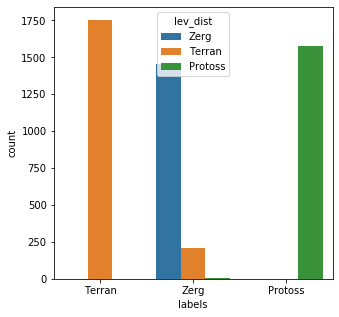
Edit Distance is clearly the better option over kmodes in this case; 4785/5000 (95.7%) of the records were matched correctly. It is also very simple to implement as an added bonus. One issue that you should be aware of when using edit distance, is that it can have a tendency to overweight noise. What I mean by this is that since Edit distance simply counts additions, subtractions, and deletions required to transform a word into another, for shorter words even moderate levels of noise can overload the metric. You can see a glimpse of this when looking at the middle category in the above chart. The same also holds true for distinguishing between words that are similar. For example:
print(dist('Terran','Terran Incorporated'))
print(dist('Terran','Tread Incorporated'))13
13
In the above example, Edit Distance does not provide any guidance at all. This is in the best case where there are no misspellings to muddy the waters even further. The more categories you have, the more difficult the situation becomes. While Edit Distance performed well here, across a large volume of data with diverse issues don’t expect it to give you the best answer. Let’s continue our exploration.
Candidate 3: Cosine Similarity
Cosine similarity measures the angle between two vectors. Since we’ve already transformed the words into vectors this should be a relatively easy transition and should provide some interesting results. We’ll calculate the cosine similarity of each element in the messy list to each of our keys and return the highest value.
from sklearn.metrics.pairwise import cosine_similarity

key_vec = [x.lower() for x in key_set]
key_vec = vec.fit_transform(key_vec).toarray()

results = []
for rec in bad_child_vec:
    cosim = [cosine_similarity([rec],[x]) for x in key_vec]
    results.append(key_set[cosim.index(max(cosim))])

messy_df['cosim'] = results
messy_df['cos_eval'] = [a == b for a,b in zip(messy_df['cosim'],messy_df['labels'])]
messy_df['cos_eval'].describe()count     5000
unique       2
top       True
freq      4935
Name: cos_eval, dtype: objectplt.subplots(figsize = (5,5))
sns.countplot(
    x=messy_df['labels'],
    order=messy_df['labels'].value_counts().index,
    hue=messy_df['cosim']
)
plt.show()
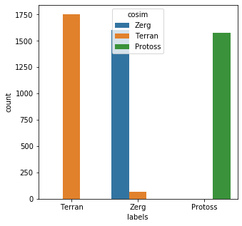
This method performed slightly better than Edit Distance; 4935/5000 (98.7%) of the records were matched correctly. The main issue to watch out for with cosine similarity has more to do with the preparation of the data itself. The vectorizer used here tokenizes the letters of each word; The actual order of letters is not taken into account. This leads to a similar issue that can plague edit distance in that shorter words are easier to miscategorize. You can see this in the above chart as well. Here is another classic example:
cosine_similarity(
    vec.fit_transform(['read']).toarray(),
    vec.fit_transform(['dear']).toarray()
)[0][0]1.0
Due to the way the words are vectorized, cosine similarity returns a perfect match for these two words with very different meanings. Let’s continue exploring.
Candidate 4: Neural Network
The last approach I wanted to explore here is a neural network with an embedding matrix. An embedding layer in a neural network tries to provide a meaningful representation of a categorical variable in space while learning relationships between the categorical variables. I’m hopeful of this approach because it should have the ability to correct for the issues presented by cosine similarity and edit distance.
from keras import layers
from keras.models import Sequential
from keras.utils import to_categorical

embedding_dim = 50
model = Sequential()
model.add(layers.Embedding(
    input_dim=26,
    output_dim=embedding_dim,
    input_length=26)
)
model.add(layers.Flatten())
model.add(layers.Dense(3, activation='softmax'))
model.compile(
    optimizer='adam',
    loss='categorical_crossentropy',
    metrics=['accuracy']
)
model.summary()Model: "sequential_4"
_________________________________________________________________
Layer (type)                 Output Shape              Param #
=================================================================
embedding_4 (Embedding)      (None, 26, 50)            1300
_________________________________________________________________
flatten_4 (Flatten)          (None, 1300)              0
_________________________________________________________________
dense_5 (Dense)              (None, 3)                 3903
=================================================================
Total params: 5,203
Trainable params: 5,203
Non-trainable params: 0
_________________________________________________________________answers = {x:i for i,x in enumerate(key_set)}
rev_answers = {i:x for i,x in enumerate(key_set)}
labels = [answers[x] for x in mr_clean]
y_binary = to_categorical(labels)

print(labels[:3])
print(y_binary[:3])[2, 0, 0]
[[0. 0. 1.]
 [1. 0. 0.]
 [1. 0. 0.]]import numpy as np

history = model.fit(
    np.array(mr_clean_vec),y_binary,
    epochs=10,
    batch_size=50,
    validation_data=(np.array(mr_clean_vec),y_binary),
    verbose=False
)x = model.predict(np.array(bad_child_vec))
results = [rev_answers[X.argmax()] for X in x]messy_df['embedding'] = results
messy_df['emb_eval'] = [a == b for a,b in zip(messy_df['embedding'],messy_df['labels'])]
messy_df['emb_eval'].describe()count     5000
unique       2
top       True
freq      4728
Name: emb_eval, dtype: objectplt.subplots(figsize = (5,5))
sns.countplot(
    x=messy_df['labels'],
    order=messy_df['labels'].value_counts().index,
    hue=messy_df['embedding']
)
plt.show()
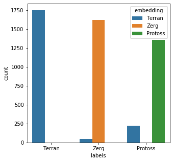
The model performed fairly well; 4728/5000 (94.56%) of the records were matched correctly. However, I think training on some messy data will improve the outcome.
training,tr_lbl = [css(x) for x in mr_clean], mr_clean*2
training.extend(mr_clean)

training_vec = [x.lower() for x in training]
training_vec = vec.fit_transform(training_vec).toarray()

labels = [answers[x] for x in tr_lbl]
y_binary = to_categorical(labels)

history = model.fit(
    np.array(training_vec),y_binary,
    epochs=10,
    batch_size=50,
    validation_data=(np.array(training_vec),y_binary),
    verbose=False
)

x = model.predict(np.array(bad_child_vec))
results = [rev_answers[X.argmax()] for X in x]

messy_df['embedding2'] = results
messy_df['emb_eval2'] = [a == b for a,b in zip(messy_df['embedding2'],messy_df['labels'])]
messy_df['emb_eval2'].describe()count     5000
unique       2
top       True
freq      4923
Name: emb_eval2, dtype: objectplt.subplots(figsize = (5,5))
sns.countplot(
    x=messy_df['labels'],
    order=messy_df['labels'].value_counts().index,
    hue=messy_df['embedding2']
)
plt.show()
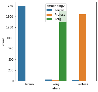
The new model performed very well; 4923/5000 (98.46%) of the records were matched correctly.
Conclusion
I think that the neural network is the most robust solution to the problem of merging disparate data sources. While some of the other solutions are simpler to implement, I think long-term the neural network will perform the best. There is some room for improvement left in the model as well, which should solidify the outcome even more. It also may be interesting to incorporate the Edit distance and cosine similarity as inputs into the neural network and see how the performance is affected. Thanks for taking the time to explore this problem with me.
You can see the notebook with the accompanying code for reference here.
About the Author

Mark Styx
I am a senior data analyst working for an international advertising agency; I specialize mainly in data engineering and mining using Python and SQL. I like to explore new ideas and ways of solving problems, and I think writing is a great tool to accomplish this.

