Two different image search engines developed with Deep Learning algorithms
Introduction
Imagine that you want to search for similar images to any picture. Imagine searching on the web for similar images to the one we are taking with our phones. In this post, we are going to develop and compare two different ways in which using Deep Learning algorithms we can solve this problem of querying between thousands of images, the most similar images.
We are going to compare two different approaches:
- Autoencoder
- Image Features Extraction
Data
We are going to solve this problem using the Flipkart images dataset. So we are going to find similar images from the products of this huge Indian e-commerce.
After downloading the images from the available URLs found on the data, we get 18322 images of different products.
The code for downloading images and developing both approaches is found on this Github repo.
Autoencoder
Let’s try to get similar images, by using an Autoencoder model. This type of model consists of three main parts:
- Encoder
- Latent Space
- Decoder
The idea behind this model, is to reconstruct the input we feed the algorithm, so the input and output size is the same. So if we can the input, we can reduce the dimension of the image, to a very small vector, and this vector is the Latent Space. If the model is robust, we can reduce all the complexity of the image to a small dimension.
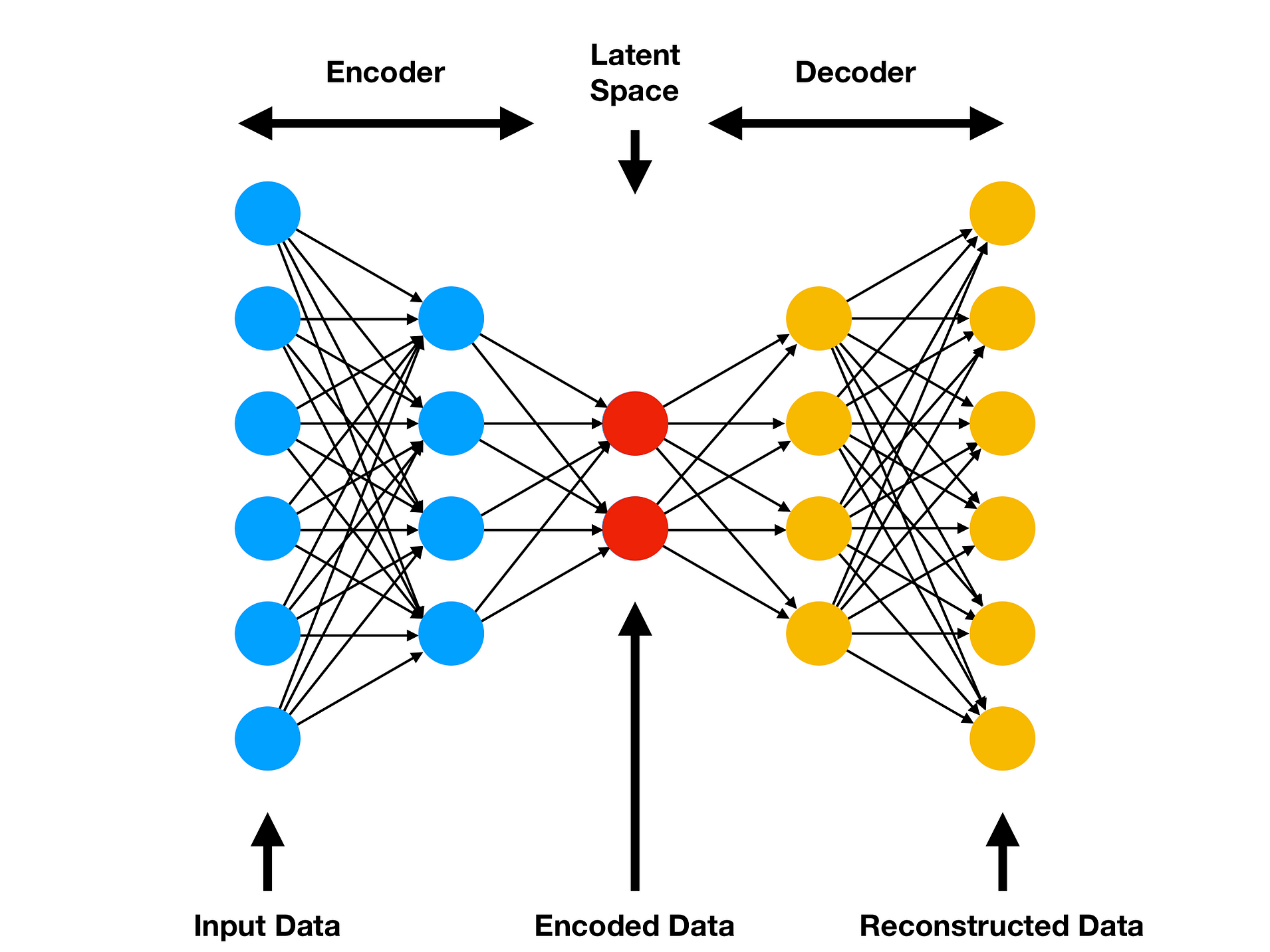
Autoencoder architecture / Source: Comp Three Inc
To train the Autoencoder, we are going to use the Keras module inside the Tensorflow 2.0 library. Once we have downloaded the images, we can define the training and validation set. Here, we are going to use the ImageDataGenerator API.
from tensorflow.keras.preprocessing.image import ImageDataGenerator, load_img, img_to_array, array_to_img
from tensorflow.keras.models import Model, load_model
from tensorflow.keras.layers import Flatten, Conv2D, Conv2DTranspose, LeakyReLU, BatchNormalization, Input, Dense, Reshape, Activation
from tensorflow.keras.optimizers import Adam
from tensorflow.keras.callbacks import ModelCheckpoint
import tensorflow.keras.backend as K
import numpy as np
import matplotlib.pyplot as plt
from tqdm import tqdm_notebook as tqdm
import pickle
import pandas as pd

# Load images
img_height = 256
img_width = 256
channels = 3
batch_size = 16

train_datagen = ImageDataGenerator(rescale=1./255,
                                   validation_split=0.2)

training_set = train_datagen.flow_from_directory(
    './flipkart/images',
     target_size = (img_height, img_width),
     batch_size = batch_size,
     class_mode = 'input',
     subset = 'training',
     shuffle=True)

validation_set = train_datagen.flow_from_directory(
    './flipkart/images',
     target_size = (img_height, img_width),
     batch_size = batch_size,
     class_mode = 'input',
     subset = 'validation',
     shuffle=False)
The argument class_mode='input' is the key here. On the ImageDataGenerator documentation, we found the following:
- class_mode: one of “binary”, “categorical”, “input”, “multi_output”, “raw”, sparse” or None. Default: “categorical”. Mode for yielding the targets: —
"binary": 1D numpy array of binary labels, –"categorical": 2D numpy array of one-hot encoded labels. Supports multi-label output. –"input": images identical to input images (mainly used to work with autoencoders), –"multi_output": list with the values of the different columns, –"raw": numpy array of values iny_colcolumn(s), –"sparse": 1D numpy array of integer labels, –None, no targets are returned (the generator will only yield batches of image data, which is useful to use inmodel.predict()).
Also, for this to work, you should have all images inside another folder, so the Keras API assumes you have only one class. In this example, I have the following images directory: flipkart/images/images/...
Now, we can define our model architecture, and fit it with the images:
# Define the autoencoder
input_model = Input(shape=(img_height, img_width, channels))

# Encoder layers
encoder = Conv2D(32, (3,3), padding='same', kernel_initializer='normal')(input_model)
encoder = LeakyReLU()(encoder)
encoder = BatchNormalization(axis=-1)(encoder)

encoder = Conv2D(64, (3,3), padding='same', kernel_initializer='normal')(encoder)
encoder = LeakyReLU()(encoder)
encoder = BatchNormalization(axis=-1)(encoder)

encoder = Conv2D(64, (3,3), padding='same', kernel_initializer='normal')(input_model)
encoder = LeakyReLU()(encoder)
encoder = BatchNormalization(axis=-1)(encoder)

encoder_dim = K.int_shape(encoder)
encoder = Flatten()(encoder)

# Latent Space
latent_space = Dense(16, name='latent_space')(encoder)

# Decoder Layers
decoder = Dense(np.prod(encoder_dim[1:]))(latent_space)
decoder = Reshape((encoder_dim[1], encoder_dim[2], encoder_dim[3]))(decoder)

decoder = Conv2DTranspose(64, (3,3), padding='same', kernel_initializer='normal')(decoder)
decoder = LeakyReLU()(decoder)
decoder = BatchNormalization(axis=-1)(decoder)

decoder = Conv2DTranspose(64, (3,3), padding='same', kernel_initializer='normal')(decoder)
decoder = LeakyReLU()(decoder)
decoder = BatchNormalization(axis=-1)(decoder)

decoder = Conv2DTranspose(32, (3,3), padding='same', kernel_initializer='normal')(decoder)
decoder = LeakyReLU()(decoder)
decoder = BatchNormalization(axis=-1)(decoder)

decoder = Conv2DTranspose(3, (3, 3), padding="same")(decoder)
output = Activation('sigmoid', name='decoder')(decoder)

# Create model object
autoencoder = Model(input_model, output, name='autoencoder')

# Compile the model
autoencoder.compile(loss="mse", optimizer= Adam(learning_rate=1e-3))

# Fit the model
history = autoencoder.fit_generator(
          training_set,
          steps_per_epoch=training_set.n // batch_size,
          epochs=100,
          validation_data=validation_set,
          validation_steps=validation_set.n // batch_size,
          callbacks = [ModelCheckpoint('models/image_autoencoder_2.h5',
                                       monitor='val_loss',
                                       verbose=0,
                                       save_best_only=True,
                                       save_weights_only=False)])
Once the model is fitted, we can try to reconstruct some images, since this is the objective of the Autoencoder:
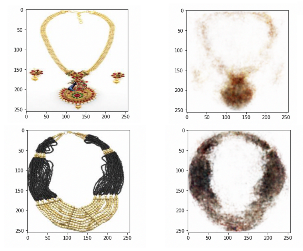
Left: image input / Right: image reconstruction with the trained Autoencoder
It is time to use Latent Space to find similar images. To accomplish this, we do not need the final prediction, we need the output of an intermediate layer, specifically, the one we named latent_space on the model definition. This is why it is important to name every layer in the model, so we can access quickly and transparently any layer we need.
Using the Model API and the .get_layer() method of the trained model is very easy to define a model with the input and output layer we choose:
latent_space_model = Model(
                      autoencoder.input,
                      autoencoder.get_layer(‘latent_space’).output)
Now every time we use the .predict() method with an image as the input of this new model, we get the Latent Space as the output.
To use this approach to get similar images, we need to predict with the latent_space_model every image, so we can compute the euclidean distance between all our saved images, and any new picture we want to find similar images.
# Load all images and predict them with the latent space model
X = []
indices = []

for i in tqdm(range(len(os.listdir('./flipkart/images/images')))):
  try:
    img_name = os.listdir('./flipkart/images')[i]
    img = load_img('./flipkart/images/images/{}'.format(img_name),
                   target_size = (256, 256))
    img = img_to_array(img) / 255.0
    img = np.expand_dims(img, axis=0)
    pred = latent_space_model.predict(img)
    pred = np.resize(pred, (16))
    X.append(pred)
    indices.append(img_name)

  except Exception as e:
    print(img_name)
    print(e)

    # Export the embeddings
embeddings = {'indices': indices, 'features': np.array(X)}
pickle.dump(embeddings,
            open('./flipkart/image_embeddings.pickle', 'wb'))
As I already stated, we are going to find similar images by calculating the euclidean distance, so the lower the value of this calculation, the higher the resemblance of the images. We define euclidean distance as:
def eucledian_distance(x,y):
  eucl_dist = np.linalg.norm(x - y)
  return eucl_dist
Once we have everything defined, we can get the three most similar products of any input image. For example, if we input the following Polo shirt, we get the following 3 most similar objects:
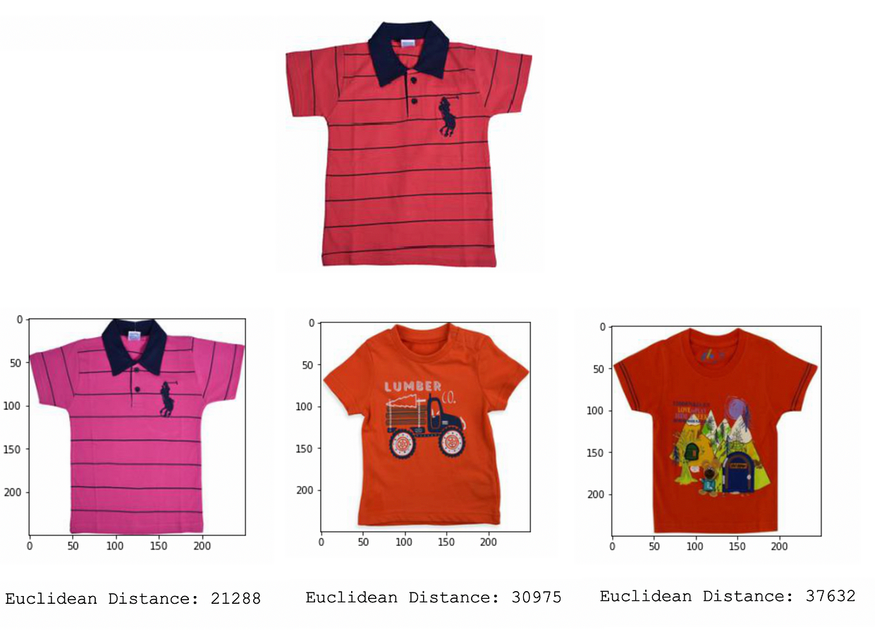
Input image and 3 most similar
Image Feature Extraction
Another approach to solving this problem is to calculate the distances to the image features. Here we can use a pre-trained Deep Learning model, to extract every image features and then compare them to any new picture. In that sense, this approach is not quite different from that of the Autoencoder model, but what is very different, is the model architecture we are going to use.
In this case, we are going to use a VGG16 pre-trained model on the imagenet dataset
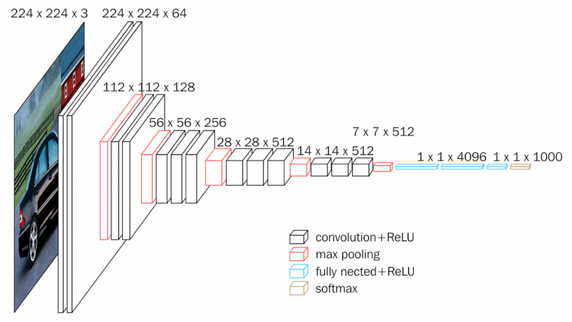
VGG16 architecture / Source: neurorhive.io
Here we are not going to train the model, we are going to extract the image features, by getting the output of the fully connected layer (named fc1).
We define the following class to extract the features of the images
from tensorflow.keras.preprocessing import image
from tensorflow.keras.applications.vgg16 import VGG16, preprocess_input
from tensorflow.keras.models import Model
import numpy as np

class FeatureExtractor:
    def __init__(self):
        # Use VGG-16 as the architecture and ImageNet for the weight
        base_model = VGG16(weights='imagenet')
        # Customize the model to return features from fully-connected layer
        self.model = Model(inputs=base_model.input, outputs=base_model.get_layer('fc1').output)

    def extract(self, img):
        # Resize the image
        img = img.resize((224, 224))
        # Convert the image color space
        img = img.convert('RGB')
        # Reformat the image
        x = image.img_to_array(img)
        x = np.expand_dims(x, axis=0)
        x = preprocess_input(x)
        # Extract Features
        feature = self.model.predict(x)[0]
        return feature / np.linalg.norm(feature)
Once we get the output of every image, we can choose a picture and get the top 3 most similar images. If we compare the same Polo shirt we used with the Autoencoder model, we get the following results:
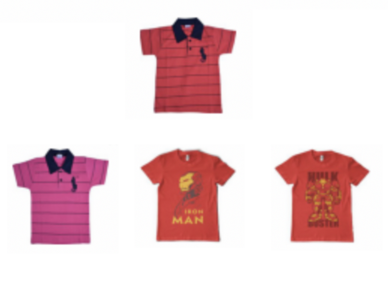
The input image and 3 most similar
As we can see, these results are not so different from the previous approach.
Conclusion
In this post, we compared two different approaches to develop an image search engine and get image results by using a picture as an input.
We developed an Autoencoder and an Image Feature Extraction approach and get very similar results.
About the Author

Luciano Naveiro
Actuary and Data Scientist.
I love the way we can explain and model the world by using math and statistics.
Buenos Aires, Argentina
The media shown in this article are not owned by Analytics Vidhya and is used at the Author’s discretion.


Hi Luciano, I was trying to implement your first solution but at the end I don't see how to finish this solution. What is x and y in the eucledian_distance function? Could you please advise me in how to finish this method? Thanks, Erick