Introduction:
Hello Readers!
Ever wonder what are the factors which govern our stock indices. There are a lot of factors involved but we will try to analyze one such factor today. In this analysis, we will try to analyze the impact of foreign stock indices on the Indian stock market. In our country, we have two main stock indices but for the sake of our analysis, we will do all our analysis on Sensex. We will analyze the impact of a variety of indexes that are of both developing and developed economies.
Contents
- The objective of the Analysis
- DataDescription
- Challenges with the available data Correlation Matrix
- Granger Causality Test
- Conclusion
The objective is to test whether there is any association of Sensex with Dow Jones Industrial Average, FTSE, Nasdaq, S&P 500, Nikkei 225, DAX PERFORMANCE-INDEX, CAC 40, FTSE MIB, Bovespa Index (Brazilian), ASX 200, and KOSPI.
Data Description
Closing prices of 12 indices (Sensex, Dow Jones Industrial Average, FTSE, Nasdaq, S&P 500, Nikkei 225, DAX PERFORMANCE-INDEX, CAC 40, FTSE MIB, Bovespa Index (Brazilian), ASX 200and KOSPI) are considered for a period of 15 years which is from January 2007 to April 2021.
Challenges with the available dataTime series such as stock indices contain components of trend and seasonality which can massively impact the statistical analysis.
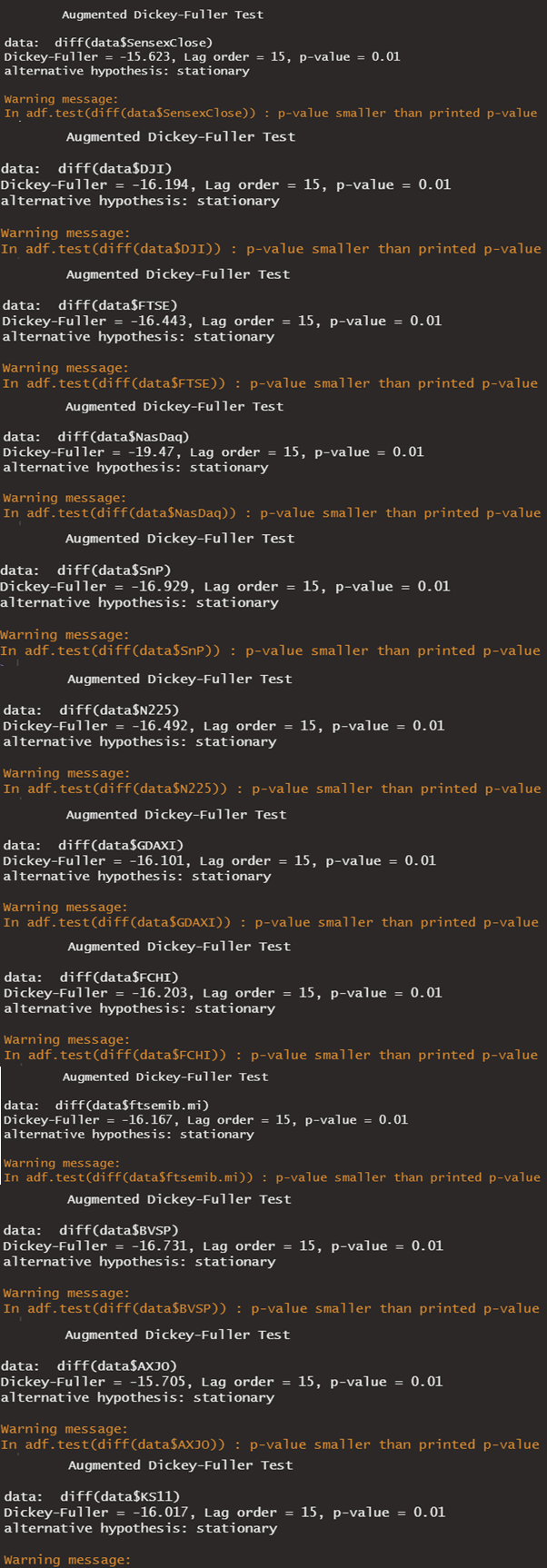
Series Stationery: In order to have a fair comparison in correlation analysis we converted all-time series into stationary. Differencing is the technique used, as single differencing the time series helped the series to remove the trend and make it stationary. Differencing is nothing but taking a difference of two consecutive terms in a time series. The stationarity of a series is tested by augmented Dickey-Fuller test (with adf.test() function from series package in R).
Augmented Dickey-Fuller test (ADF) tests the presence of a unit root in a time series sample and the alternative hypothesis of the test: series is stationarity.
Definition of Stationary: a time series that does not show a trend and seasonality in it.
Dataset
data<-read.csv("world_index.csv")
Test stationarity
adf.test(diff(data$SensexClose))
adf.test(diff(data$SnP))
adf.test(diff(data$N225))
adf.test(diff(data$GDAXI))
adf.test(diff(data$FCHI))
adf.test(diff(data$ftsemib.mi))
adf.test(diff(data$BVSP))
adf.test(diff(data$AXJO))
adf.test(diff(data$KS11))
adf.test(diff(data$DJI))
adf.test(diff(data$FTSE))
adf.test(diff(data$NasDaq))
#Output

Correlation Matrix: correlation is calculated of each time series taking two at a time to create a correlation matrix.
#correlation_matrix
cor_mat<-cor(data_new)
corrplot(cor_mat,diag = F,method = "square",type = "upper",bg="white")
| Correlation with Sensex | Correlation |
| Sensex with Dow Jones Industrial Average | 0.5038221 |
| Sensex with FTSE | 0.103973 |
| Sensex with Nasdaq | 0.4084861 |
| Sensex with S&P 500 | 0.4385984 |
| Sensex with Nikkei 225 | 0.5644592 |
| Sensex with DAX PERFORMANCE-INDEX | 0.3130041 |
| Sensex with CAC 40 | 0.4668009 |
| Sensex with FTSE MIB | 0.4591162 |
| Sensex with Bovespa Index | 0.510072 |
| Sensex with ASX 200 | 0.6134182 |
| Sensex with KOSPI | 0.3923573 |
From the correlation analysis, we observe a correlation between Sensex and the following indices of more than 0.5 ASX 200 (Australia), Bovespa Index (Brazil), Nikkei 225(Tokyo Stock Exchange), and Dow Jones.
Granger Causality Test: Granger causality test shows the impact of one series on the other. For example, the impact of the increase in house prices in certain areas triggers the increase in prices of houses in all nearby areas in subsequent months or years.
#Granger_causality_lag=1
grangertest(data_new$Sensex,data_new$Dow)
grangertest(data_new$Sensex,data_new$FTSE)
grangertest(data_new$Sensex,data_new$Nasdaq)
grangertest(data_new$Sensex,data_new$SnP)
grangertest(data_new$Sensex,data_new$N225)
grangertest(data_new$Sensex,data_new$GDAXI)
grangertest(data_new$Sensex,data_new$FCHI)
grangertest(data_new$Sensex,data_new$ftsemib.mi)
grangertest(data_new$Sensex,data_new$BVSP)
grangertest(data_new$Sensex,data_new$AXJO)
grangertest(data_new$Sensex,data_new$KS11)
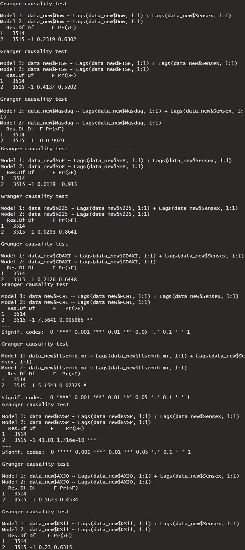
#Output

| Granger Causality Test | F-Value | P-Value | Status |
| Sensex with Dow Jones Industrial Average | 0.2319 | 0.6302 | Insignificant |
| Sensex with FTSE | 0.4137 | 0.5202 | Insignificant |
| Sensex with Nasdaq | 0 | 0.9979 | Insignificant |
| Sensex with S&P 500 | 0.0119 | 0.913 | Insignificant |
| Sensex with Nikkei 225 | 0.0293 | 0.8641 | Insignificant |
| Sensex with DAX PERFORMANCE-INDEX | 0.2126 | 0.6448 | Insignificant |
| Sensex with CAC 40 | 7.5641 | 0.005985 | Significant |
| Sensex with FTSE MIB | 5.1543 | 0.02325 | Significant |
| Sensex with Bovespa Index | 41.01 | 1.716e-10 | Significant |
| Sensex with ASX 200 | 0.5623 | 0.4534 | Insignificant |
| Sensex with KOSPI | 0.23 | 0.6315 | Insignificant |
From the Granger causality test, it is clear that the indices which are causing movement in Sensex are CAC 40(France), FTSE MIB(Italy), and Bovespa Index(Brazil).
Conclusion
From the above analysis, we understood that Sensex closing prices are associated with other world indices. The information can be further utilized to fit a time series model such as Vector Auto Regression (Vector autoregression (VAR) is a statistical model used to capture the association between multi-variate time-series. VAR model’s applications are mostly in economics and the natural sciences) to predict the closing prices for Sensex.
The media shown in this article are not owned by Analytics Vidhya and is used at the Author’s discretion.


This is a very useful emphasis. Thank you
If Test statistic < Critical Value and p-value Test statistic < Critical Value - Reject Null Hypthesis - Data is stationary
What if both tests tell me my data is stationary but when I look at the graph it is obviosly non-stationary?